注意力替代方案与专家混合

01 开场：注意力为什么贵

0:17 you should be able to get it through the course website. But if not, it's definitely up there on the GitHub. Today we're going to talk about what I think of as kind of like more advanced architecture ideas. So, last lecture was really about the basic transformer and how we might tweak different parts of the basic transformer to get to a modern language model. Now I want to talk about things that I think are much more advanced, much more complex developments on top of the usual transformer. And the two things I'll talk about today, the first one is attention alternatives, ways of going to much longer contexts using architectural changes that for the most part generally allow for linear time dependence on the length of the sequence rather than quadratic. The second thing I want to talk about is the idea of mixture of experts. Right? So, the first part is modifying the attention block. #

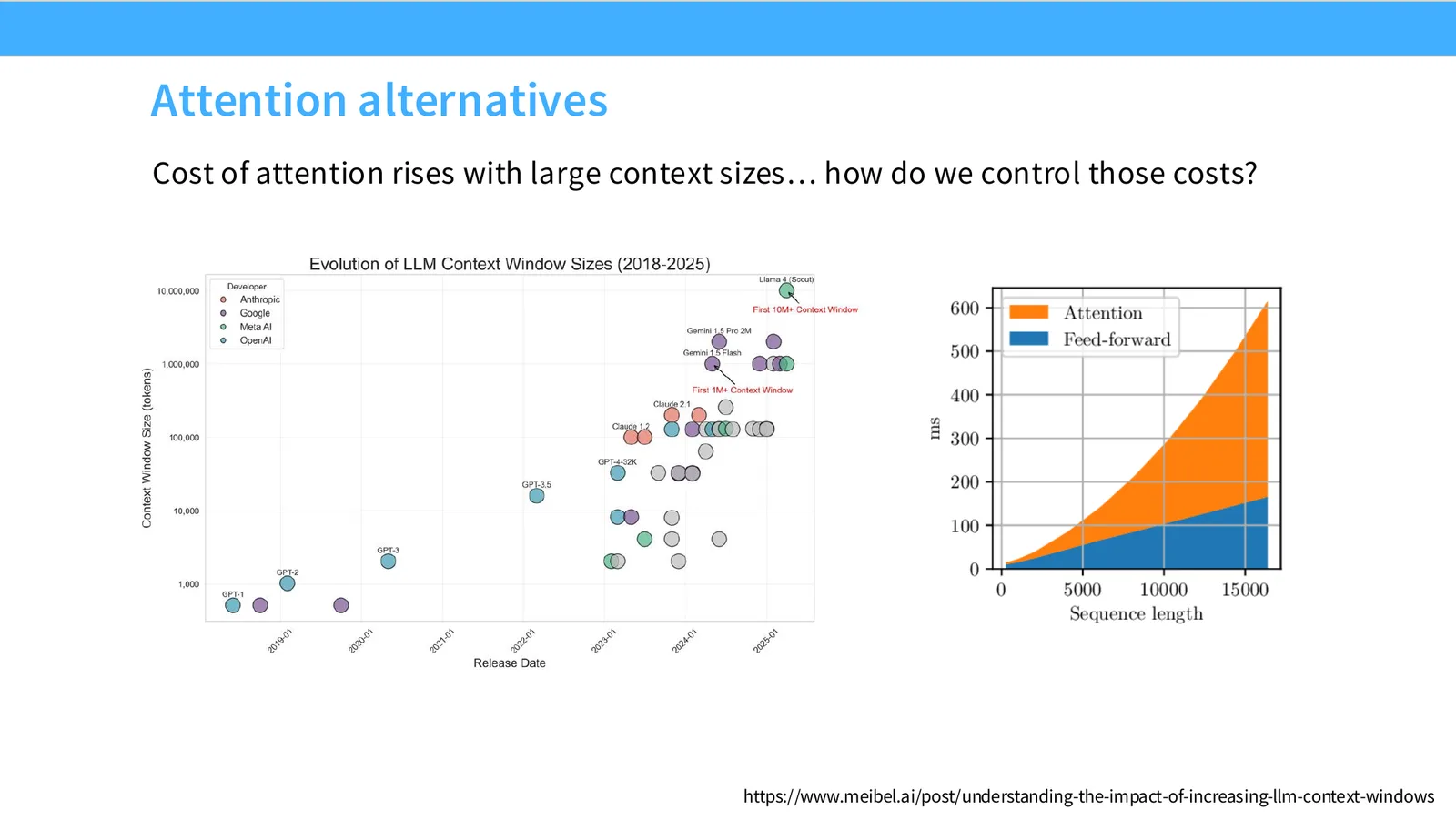
1:13 The second part is going to be modifying the MLP part. Right? A mixture of experts are going to give us significantly better utilization in terms of our hardware, in terms of having more parameters relative to the compute that we have to spend on these models. So, those are the two parts and the two ideas for today. So, I'm going to start with attention and I'm going to set the stage. It's clear now that people want longer context length. Right? You want to pack a lot of things into the context so that your model has more knowledge, maybe it's an agent and operates on lots of things. If you look at, you know, different models over time on the x-axis over here, and you know the context window size, this is in log scale, you know, there's really a clear rush by a lot of the top LM vendors that provide larger and larger context sizes to support these kinds of, you know, more complex workloads. #

2:05 Now, how do we control these costs? Well, you know, not yet. The right plot also shows, you know, the ratio between, you know, how much compute cost is spent in the feed forward part of the network versus the attention part of the network as you increase the sequence length. And you see that, you know, the feed forward fairly large at the start, but grows linearly. Attention, right, is an all-to-all connection between all the different positions, quadratic, so quickly outpaces feed forward as the sequence length grows, right? So, you know, it used to be that for big models that like smallish sequence lengths, feed forward was the dominant cost. #

02 基础工具箱：局部/全局注意力与 FlashAttention

2:41 As you go to these longer sequence lengths, attention increasingly becomes more and more of a problem, right? #

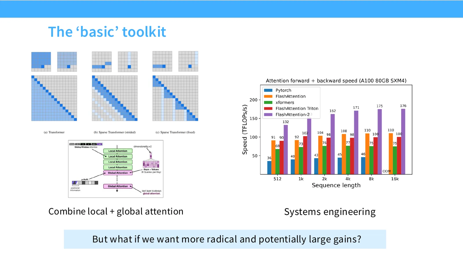
2:49 Now, what's kind of the basic toolkit by which we can control these? And we've already talked about these, or well, we talked about one of these, and we will talk about another one of these. You know, we can basically take things like local attention and combine them in different kinds of hybrid ways to control the very high cost of global attention, right? If you're only doing global attention once every eight layers and all the other ones are these like very local attentions, you've very much controlled the cost. The other thing you can do is systems engineering. I think a very underappreciated fact is, you know, constant factors really, really matter, right? Part of the theme of this course is you need to pay attention to the details. And it's very easy for people trained in like a more classical theory oriented computer science tradition to be like, ah, yes, it's the big O that matters, right? Linear or quadratic. #

3:41 But I think one of the biggest things that has happened to, you know, context and like attention cost is flash attention, right? Flash attention, we'll talk about this in a lot more detail once we get to the systems lecture and as you do the systems assignments. But flash attention is really just a very clever way of rearranging the attention operation into a much more systems friendly way to minimize memory sort of transfer overhead. And by doing so, you can get truly, truly dramatic improvements in the performance of your attention. So, you know, base PyTorch is this blue, you know, you can just kind of look at some of the shorter sequence lengths. You're doing like 30 to 40, flops per sec, a teraflops per second. and then you do flash attention, which is really a constant factor systems improvement. And you're getting these big, big improvements, like factors of two improvements. And at some sizes, you can't even fit this in memory anymore. #

4:34 But with flash attention, where you're not materializing these big attention matrices anymore, you can continue to run these. Albeit, you know, somewhat slowly, right? This doesn't fix any of the quadratic cost issues, but constant factors are very, very powerful. Now that said, you know, if we're going to, to five, 10 million tokens, these tricks might not be enough. We want much more radical, much larger gains in our ability to handle long context. So this leads us to the question, is there ways for us to have linear time or linear dependence on the length of the sequence? And what would those kinds of things, look like? Okay, there you go. it turns out that, you know, a lot of people have tried a lot of different things over the years. #

5:20 and I think there are a few false starts. but in the recent years, I would say the last two-ish years, there's been kind of an emergence of a set of recipes that are fairly effective in linear time attention. That are now kind of battle-tested at scale. and that's kind of why, this is finally the first year when I'm, you know, talking about linear time attention. Because it's clear now that these things really work at scale and in production and so on. #

03 线性注意力：结合律与循环形式

5:46 to really, explain all of these different methods that work well, I think you need to really only understand one core idea to start with. And then we're going to elaborate and build upon that idea. and that idea to start with is the associativity, of multiplication. So, let's think about how attention works. we can write it in this compact notation where we say, you know, the attention operation is going to be of q, k's, and v's, right? With these, you know, matrix dimensions up here. and you know, I'm going to take my q's and the k's and I'm going to have an all-to-all interaction, right? All the end positions are going to interact with each other by matrix multiplication. And then I'll normalize them through a soft max, this, this row over here. #

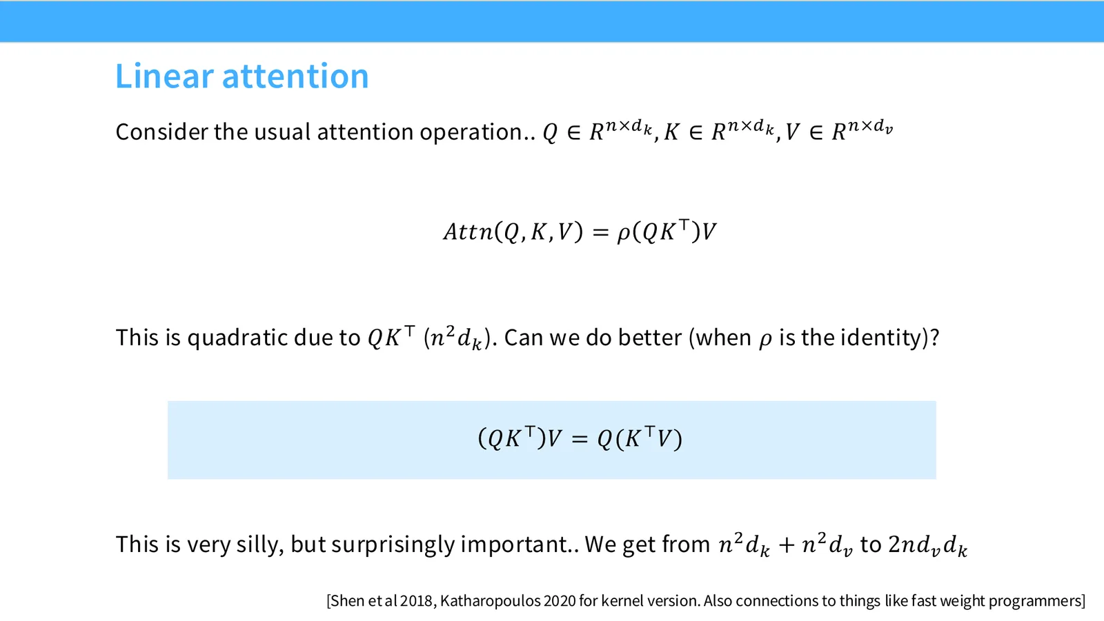
6:26 And then I will multiply it with my, my, my values v to get the attention outputs, right? This is a classic, you know, self attention or whatever other attention operation. Now, you know, for the moment, let's forget that, you know, attention has a soft max. And then I'm just going to drop the row, like forget it for the moment, right? Now, if we didn't have a row, maybe we can actually change the complexity of this operation. So, you know, if you look at attention, it's, you know, n squared dk, right? Because we're taking this q, k transpose multiplication. But if row was the identity, I can just move the parentheses around a little bit. And I can say, all right, instead of, you know, q, k transpose v, really, I'm going to have, what I'm going to have is q, k transpose v, right? #

7:09 And if we do this reordering, well, we've like changed which part is quadratic, right? Like instead of having the n squareds, which were pretty terrible because these n's are very big. They're millions, right? That's the context length. Instead, I can have dependence on n dvdk, right? So now we're multiplying essentially the key and the value dimensions. These could be big in principle, right? I can have a big model. But these are usually on the order of like thousands, tens of thousands, right? #

7:36 No one has like a million coordinates in their hidden dimensions. And so, you know, this is a much more favorable sort of, you know, term to be dependent on compared to this n squared term when we were, you know, doing this original attention operation, right? So this is the first thing that you should know, which is like associativity of multiplication allows us to change kind of the dependence on the sequence length. Okay. #

8:06 Now, the other thing that we can do now is, you know, if we consider this reordering, this like q k transpose v, something that's even nicer about this, and I think this has led to really a lot of the research that, you know, I'm going to mention in the next couple of slides, is that, you know, this matrix multiply on the right in the self-attention case looks just like an r and n, right? Instead of writing it in this dense form up here, I can write it incrementally as I sweep left to right on my context, you know, I can multiply my k's and v's, right? And I can update this thing s, which is a state, and I can add it to my previous state. This is kind of like incrementally multiplying and accumulating my k v's, and I can multiply it with my q to get my output, right? And this, you know, dense operation up here, and this r and n form, you know, are kind of equivalent. And so, you know, what have we done? Well, we've started from linear attention on the top left, and then we've somehow gotten something that looks very much like an r and n. And what's nice about r and n's, well, r and n's are quite nice because at inference time, right, I have this s, which is my state, you know, it's fixed in size, and I'm just carrying that forward and forward, right? So r and n's are very nice for inference reasons, they are, you know, not nice for training reasons, but nice thing about linear attention is you can use them in either way, right? #

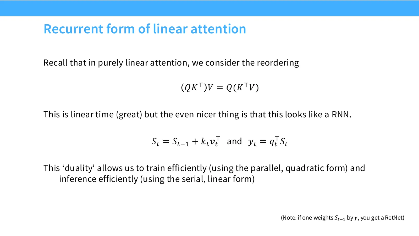
9:26 You can have it in this dense form, which will be great for training, it's parallel, or you can have it in this sort of serial form like an r and n, which is great for inference, right? So you can get the best of both worlds. Now, at least in terms of like dependence of all these objects, this is great, this is lovely. Unfortunately, this is linear, which is not very good. You know, this is really sort of a starting point of our discussion. Any questions so far? This is really the basics. #

04 线性注意力实践：MiniMax M1 / Mamba-2 / Nemotron 3

9:51 Okay. #

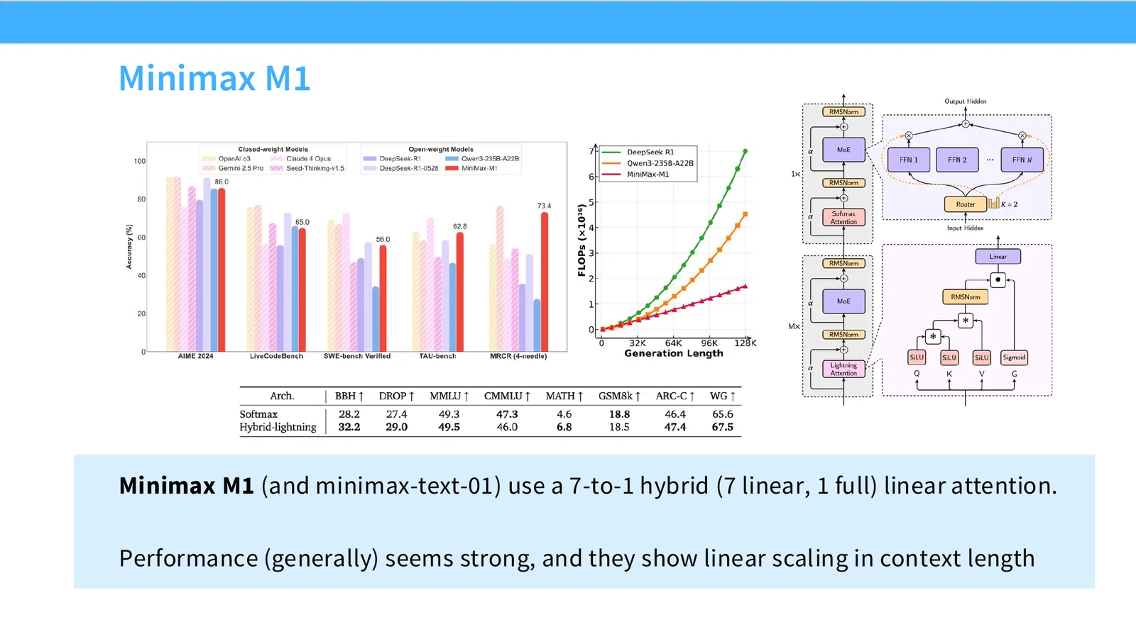
9:55 One cool thing is there have been people that have basically used this linear attention as part of their attention mechanism. So minimax M1, which is a fairly large scale, fairly high performance Chinese open model. It uses a seven to one hybrid. So seven, you know, linear attention layers plus one full soft max attention. Performance generally strong, you can compare it to a number of, you know, strong models like, you know, opening ISO three or deep sea car one, fairly competitive. And then, you know, since it's linear attention, most of the dependence on context length is linear. You know, it's not fully linear because you've got these soft maxes, but the dependence is much, much milder, right? #

10:42 So, you know, this is one example where people have shown that this, even this basic linear attention, which is very, very simple to understand, can be, you know, used fairly effectively at scale. As long as you've got some sort of full quadratic connections involved. No one has thus far really proven out fully linear time attention mechanisms at scale. Everything that I'm going to talk about in the next couple of slides is a hybrid. Okay. So now, you know, we've done linear attention, but you might say linear attention is too naive and simple for me. Like, this is not what I want. I want some more like serious, complex, neural network stuff to be happening. Well, what you can now do is, oh, sorry, went a little too far. #

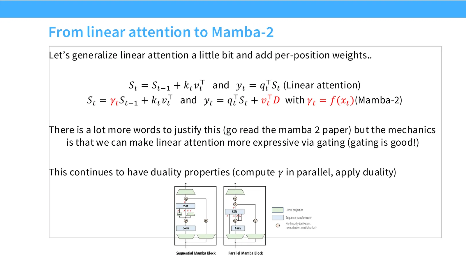
11:31 Look at the RNN form of linear attention. So, you know, I've put the linear attention equation right here just so you don't have to keep going back and forth. And we can add a small elaboration to linear attention in order to get more expressive updates. And this is how you end up getting Mamba 2. Some of you may have heard of Mamba, Mamba 2, Mamba 3 now, I think. These are a family of state space models by Albert Gu and Tri Dao and friends. And, you know, they're derived originally from like this kind of state space theory and view. But actually, if you look at the mechanics of, you know, what is being done, you can actually see it as a very simple elaboration of the linear attention mechanism. And so the idea is the following, right? #

12:16 So we start with linear attention. And you might say, really the main problem with linear attention is that I'm always passing my state forward, right? We know from like the olden days of LSTMs that it's important to know when to pass information forward and when to just not pass information forward, right? To forget things and send them to zero. So what I'm going to do is I'm going to be inspired by that. And I'm going to add a gate gamma, right? Gamma of t. Gamma of t is not stateful. Gamma of t only depends on my current inputs x of t. #

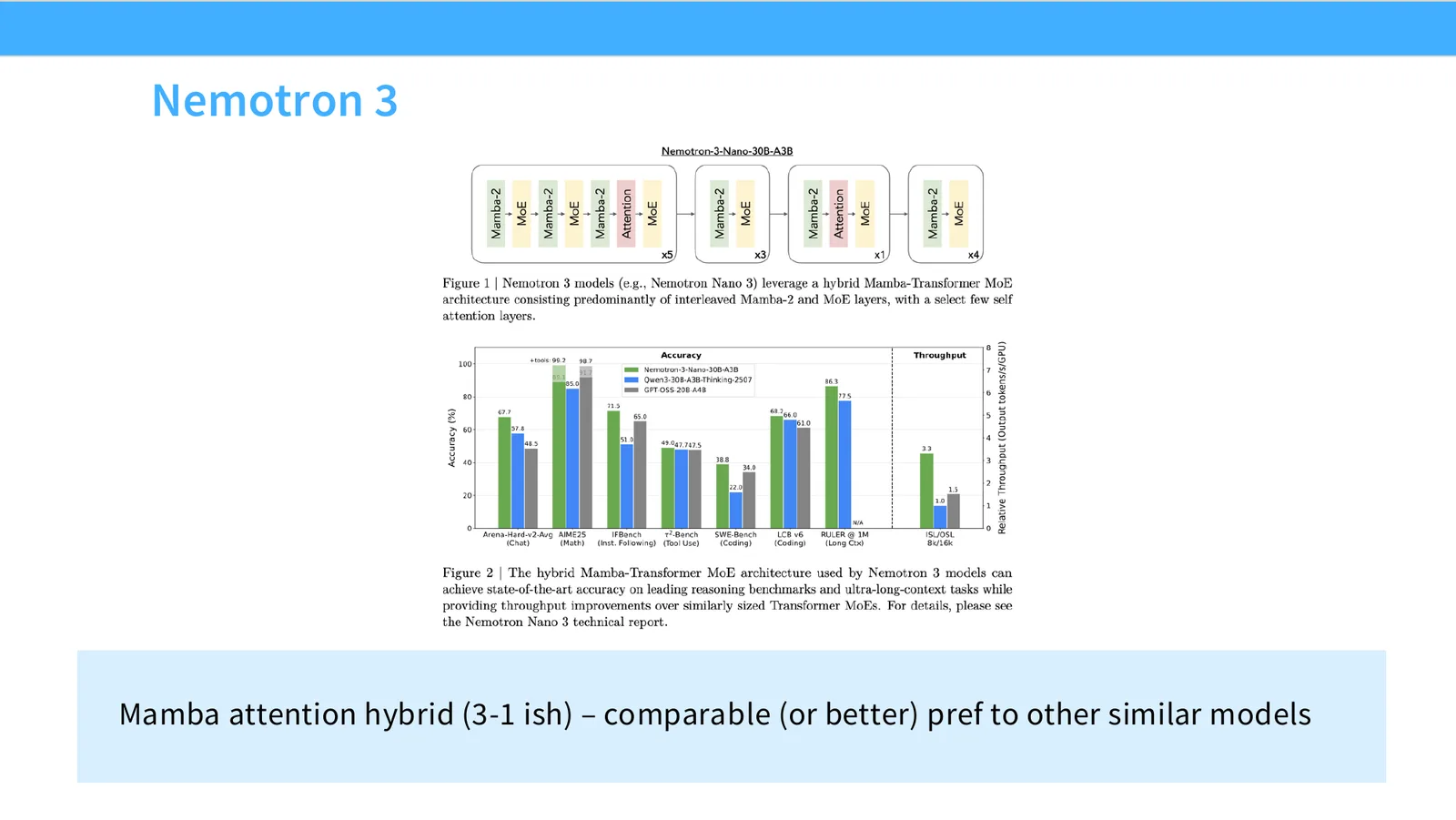
12:46 And gamma of t is going to modulate how much of my state I'm going to carry forward into the future. Now, if you think about this, you know, the state dependent terms are all these s's. This gamma is not state dependent at all. So this means that, you know, this is very simple to compute. And there's still sort of this duality. You can compute this Mamba two term either as a big dense matrix multiply or at inference time use it in this sort of recurrent form to get nice inference improvements, right? So that's kind of the core sort of conceit or view of this idea that, you know, you can either use it in parallel or sequence just like linear attention. And people have now used this at scale. So Nematron three, I mentioned briefly last lecture, uses this idea of combining Mamba two as their sort of lightweight layer. #

13:37 And of course, you've got your big soft max attention every now and then. And they sort of alternate this in various ways to manage their inference cost expressiveness trade off. #

13:49 Nematron three achieves, you know, pretty good performance compared to QEN three thinking as compared to GPT OSS. And because of all these Mamba two layers, you know, has pretty good throughput at fairly large context length. So, you know, you can see that it kind of works. At least these are small frontier models, not like really big frontier models, but, you know, small frontier models that are open source. Cool. So now we've like built on this gating idea, which is cool. You might say though, like, can we just, you know, keep pushing this idea further and like taking this recurrence and making it sort of increasingly more complex. #

05 Gated DeltaNet / Qwen Next / 混合比消融

14:31 And kind of the rule of thumb in some sense for what you can do with your operations here is as long as you're gating the various terms in your RNN, so to speak, with only input dependent terms. So no state dependence, then you'll still have this fairly nice duality between sort of parallel operations, which you can use for training and serial operations, which, you know, you are going to use for inference. So gated delta net is probably among the most widely used, I would say, states based model now. I think it's been tested in quite a few papers. And there's, you know, a very nice sort of large scale scale up in QN3, sorry, 3.5 for these models. So let me talk you through what gated delta net is in comparison to Mamba two. So Mamba two is, you know, as I have at this top here, we take the linear sort of recurrence, the state update. And what I'm going to do is I'm going to gate it with my gamma, right? #

15:33 Oh, I forgot to explain this VT, sorry, I apologize for that. I added this for completeness. Mamba two also has a modification where they add what is basically a residual layer to the YT update. It's not really core to sort of the state update or their arguments for why this is a good idea, but I put it in for completeness just to make sure I'm actually giving the true Mamba two. Updates rather than sort of a more abridged version that only gets the core ideas across. Okay, but you can ignore the VT for now. This is really just like a architectural improvement that's not core to the state updates. Gated delta net takes this idea in some sense and adds a second gate, beta t. So what does beta t do? #

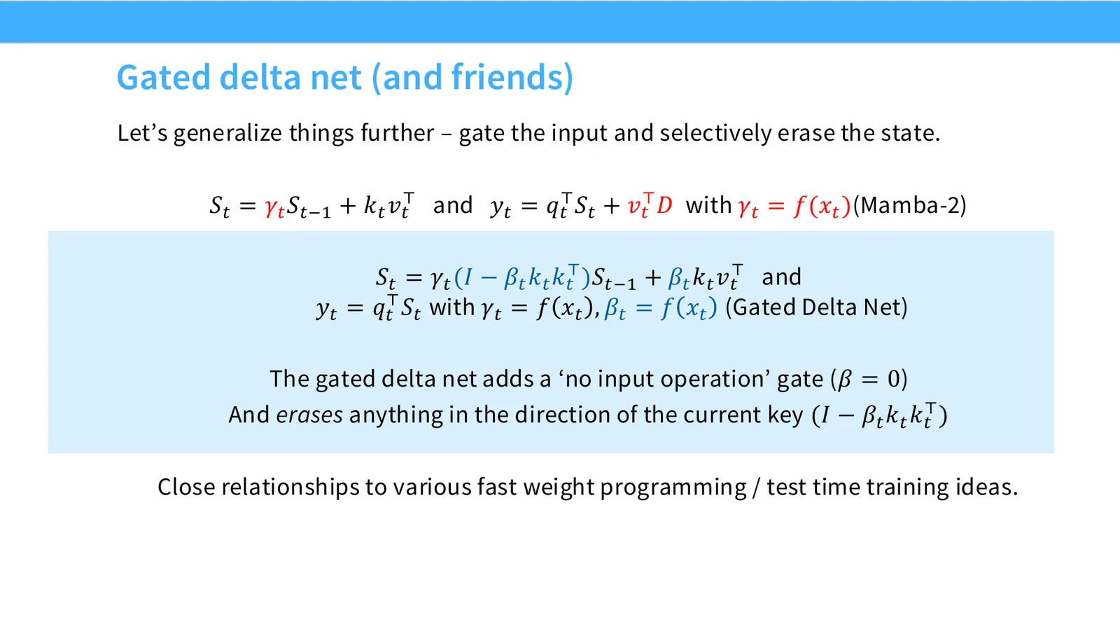
16:13 Beta t I think of as a no input operation gate, right? If beta t is zero, that basically means don't take any of my current information, don't add it into my state, right? And I think most or all of you are probably familiar with LSTMs, right? This is very reminiscent of the ideas in LSTM. You've got gates that control, you know, whether to forget and whether to put in information from the current time step, right? So it operates in a very similar set of principles. Although, of course, derived, I think, originally in a very different way. Now, the other thing that's interesting about gated delta net, and this comes from the delta net rather than the gated delta net, is this update direction. So instead of just gating things, you could have made this 1 minus beta t, for example. #

17:00 What they do is if you're going to do an update where you're putting in this beta, what you're going to do is you're going to try to project out, in some sense, my current key direction. So the intuition here is I'm going to be writing in information from my current key, k of t. And when doing that, not only do I want to put in new information, I also want to erase any previous keys that have gone into it, right? That's one way that you can think about updates, like not just put stuff in. You know, I want to clear out the current key that has gone in. And that's why there's this blue term, this identity minus beta t, kt, kt transpose, which is essentially acting as a projector that is projecting out things in the kt dimension. That's not exactly right because you're not doing things like unit normalization, but you kind of get roughly the intuition here. The other thing I'll mention before I kind of move on, oops, sorry, I have this blue box here. I'll move on with gated delta net is that this has been reinvented in some ways in various settings. #

17:57 This update, this projector appears if you try to solve certain kinds of like meta learning least squares problems. So it's been reinvented in other forms in fast weight programming or test time training, where essentially through very different design principles, researchers from those areas have basically ended up with the exact same kinds of solutions. #

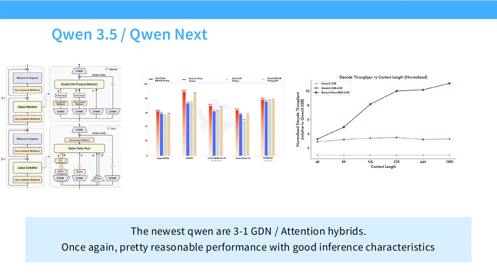
18:21 And the thing that I'll say here is, you know, the QN 3.5 and the QN Next models that were kind of predecessors to that, some of the best open source models available today. And they use exactly this, this architecture. These are three to one gated delta net attention hybrid. Very good, very reasonable performance, strong inference characteristics that you can see on the right there. You know, QN Next has like much higher decoding throughput relative to QN 3 as the context length goes up and up and up. The middle panel is a comparison of performance versus various like closed source models and like previous generation models. This hybrid architecture doesn't seem to hurt performance very much at all. #

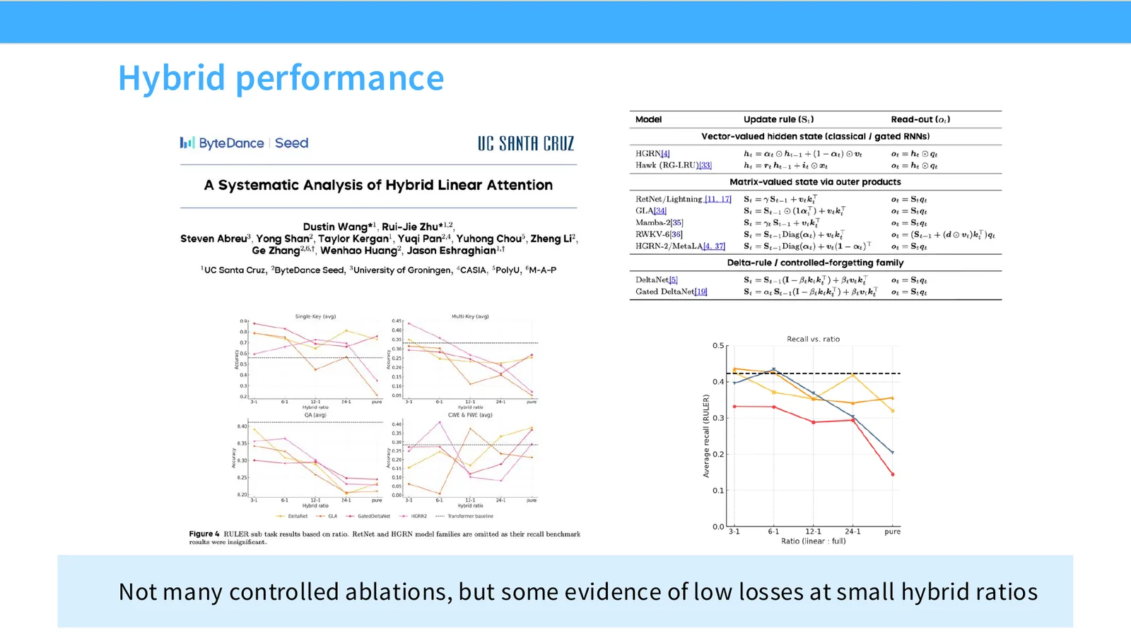
19:02 The last thing that I will say is, you know, there hasn't been that many great sort of controlled studies of how hybrid architecture is perform. There's maybe one by ByteDance Seed and UC Santa Cruz folks where they compare things like Mamba 2 and gated delta net and other architectures as a function of how many sort of hybrid layers you have. Some of the results I would say are kind of messy, but you know, the things that I would point out is this dashed line over here on this right panel. This guy is full attention performance. And as you go from left to right, this is increasing the number of sort of non full attention layers. So, you know, the RNN layers, let's call them. You know, you increase them as you go to the right and you see performance degradation. But maybe the thing to see here is that for some of the best architectures that you have, like the yellow, the orange, the blue, these are like the gated delta nets and various other variants. You know, you see that at the low ratios, there's basically no hit. #

20:01 And then, once you pass a certain point, you start to see more significant degradation in performance, in long context performance in this case. As you basically at the end, as you go to full RNN, you know, you have very noticeable performance degradation in all of these architectures. The same is true at various different other kinds of evaluations. Some of these, I think, have been optimized by the architectures themselves, like single key retrieval is a task that I think all of these long context architectures explicitly optimized for. But if you look at QA performance, we sort of see a same story. But as we increase the amount of hybrid ratio, you know, we see decreases in performance fairly steadily and fairly clearly ending up at this pure point. Okay. #

06 稀疏注意力：DSA（DeepSeek Sparse Attention）

20:42 Any questions for the linear time attention stuff? I have one last efficient attention thing to talk about, but yes. #

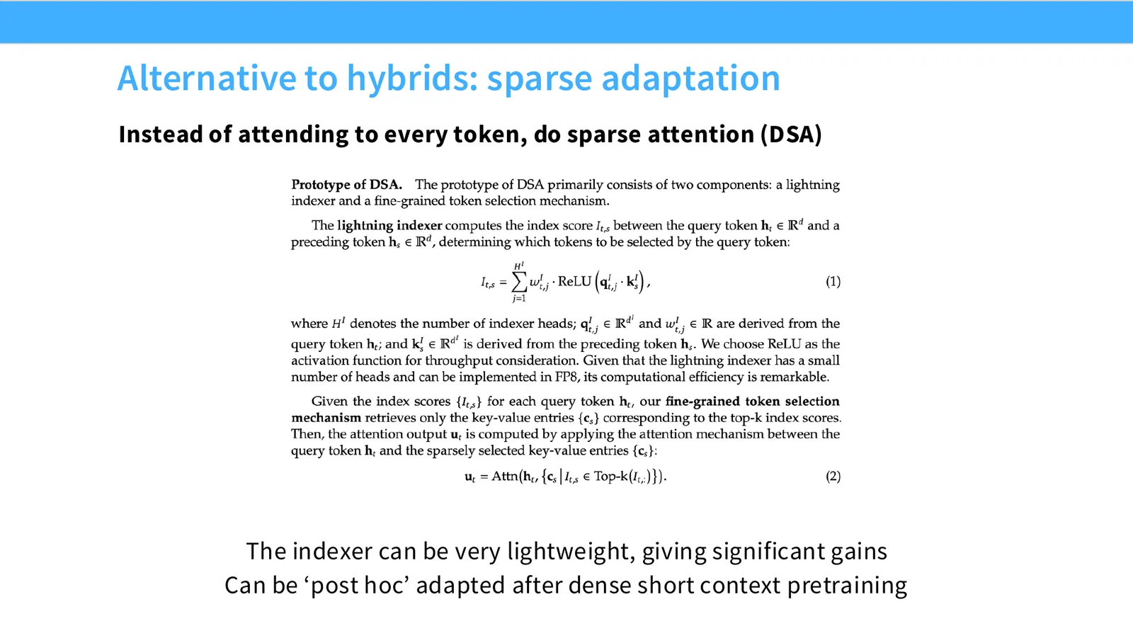
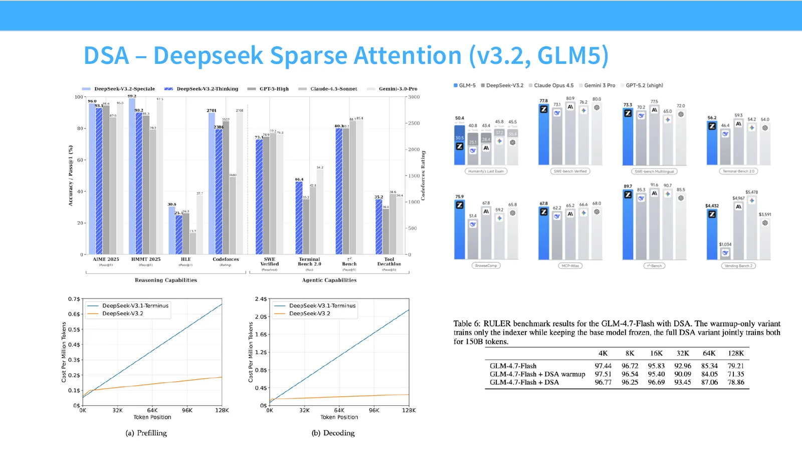
27:32 The index or the time complexity for that, is it n squared? It's quadratic. It's quadratic. Yeah. Because it has to, I mean, in order to know what to select, it does have to look at everything. Right? Okay. And there's no clever like state transition stuff that happens here. It is really brute force inner products. #

27:49 So if you're going through all of it, and then like afterwards, the step afterwards is also quadratic as well. How are we getting time to say that? I mean, it's kind of like a systems-y trick almost. Like you're going to do the indexer much more lightweight. And there are many ways to do that. You can do that in much lower precision, which they talk about. You can do it in ways that are lower dimensional by projecting the q's and k's further just for the indexing. So there are lots of tricks that you can do here that you can imagine. But the indexer is going to be much more lightweight. #

28:18 So the constant factors are very good. And then for the second one, even though it's quadratic, it's quadratic on a shorter context length. Because it's top k, we can control k. So now this is expensive, but small. So this is another one of these things of sometimes don't get too stuck up on the quadratic versus not. Sometimes the constant factors are really, really important. There's another question? Yeah. #

28:44 That's right. That's right. Or it's part of like a continued pre-training style thing. Because all the models, you don't train long context from scratch for compute and various other reasons. You train a short-ish context model first. And then you've got these long context extension stages. And so the nice idea here is that we're going to do the second phase anyway. Why don't we bolt the long context cost savings on at the same stage? And it's kind of surprising that it works. #

29:09 You know, honestly, they can bolt on this, frankly, scary looking top k non-differentiable object. But as you'll see in the next part, maybe you shouldn't be so scared of top k selection. #

29:28 Yeah, the usual recipe that I am familiar with when a lot of the open source models is it usually goes like short context pre-training, long context extension, then post-training. #

29:39 Yes? Is the k here similar in length to the short context? Yeah, that's right. You would pick values that are like much closer to short context performance. And you would bound it, right? So regardless of the input size, they would be bound. #

29:55 Actually, many questions. Okay, good. #

30:02 Training stability issues. That's a good question. I don't think so. I'm not aware of like, you know, documented linear softmax causing lots of attention. If anything, softmaxes are usually more of the problems for various reasons. So I think this will actually improve the stability properties of the architecture. #

30:24 Can you predict the next. To consider the next tree is requiring like a better, a better attention method that I need to request, because like the loop of the low community cost and the low #

30:48 Yeah, I don't know if I have good predictions for what the future attention architecture looks like. I mean, my somewhat cop-out answer to this is I think a lot of this will look like we throw all of these tricks in, right? In the same way as the architectures have gotten very complex by taking all of these successful recipes and throwing them in. I think also that there's a even broader layer or like a higher level layer of basically using post-training to have the model manage its own context, right? Compaction, retrieval, all of these things are basically an added layer on top. I think a lot of the work that I imagine will be integration of these different layers, because we've seen that, you know, at least the linear time attention stuff has converged a lot into LSTM like or linear attention like architectures. And I don't really see that changing too much in the near future. Cool. Oh, yes. #

31:43 Can you speak about like lower precision attention? Like, is FP4 attention possible? I think the indexer is partially motivated by things like this. Like FP4 attention, definitely possible. I think the drawback is that, you know, the loss of precision for things like soft maxes where like small, underflow, overflow, these kinds of things can really start to matter, can sometimes be pretty problematic. And so I think, you know, this motivation of saying like, okay, like let's do selection with low precision and then do a full precision computation afterwards. Because then the value vectors can be like more finely added together and weighted together. It's an approach that makes sense. I don't know if there's, you know, really good ways of doing full attention in FP4 or even lower precision of some kind. #

32:31 Yeah. #

32:34 Okay. Okay. Okay. Fine. One last question. #

32:39 So, compared to transformers, what's the downside? #

32:46 Is the training complicated in space? Yeah. So that's a good question. There has to be some downside. Otherwise everybody. Well, the downside I think is sort of expressive power, right? You know, the all to all connection in soft max extension is incredibly powerful. It's also very easy to train, right? It used to be, I think, you know, compared to say an LSTM, attention had the very strong advantage of like hardware efficiency, right? #

33:09 You could train in parallel. I think the reason why these state space models have caught on, you know, despite their similarity to LSTMs and similar drawbacks in terms of representational power, is that now, you know, there's this kind of well understood duality because of the linear attention sort of thing that I talked about. Where you can go from, you know, this RNN form to the more dense matrix multiply form. And the matrix multiply form allows for computational efficiency. So, you know, that trade-off has now been sort of checked off. But you've still got the trade-off of if you have a finite state and you have to carry everything through, you know, you're going to be losing some information relative just carrying everything. #

33:50 So, you know, the context itself, the transformers, is something more in state space. Well, in state space, you have to basically kind of think about the context length relative to the size of your state, right? I mean, if you have the state the size of your context, then you're good to go. But then you're paying these like very large costs, right? So, really the point is, the free lunches, if you want a really tiny state, it's really hard to compress all the information in a big context, right? #

07 MoE 引入：是什么、为什么流行

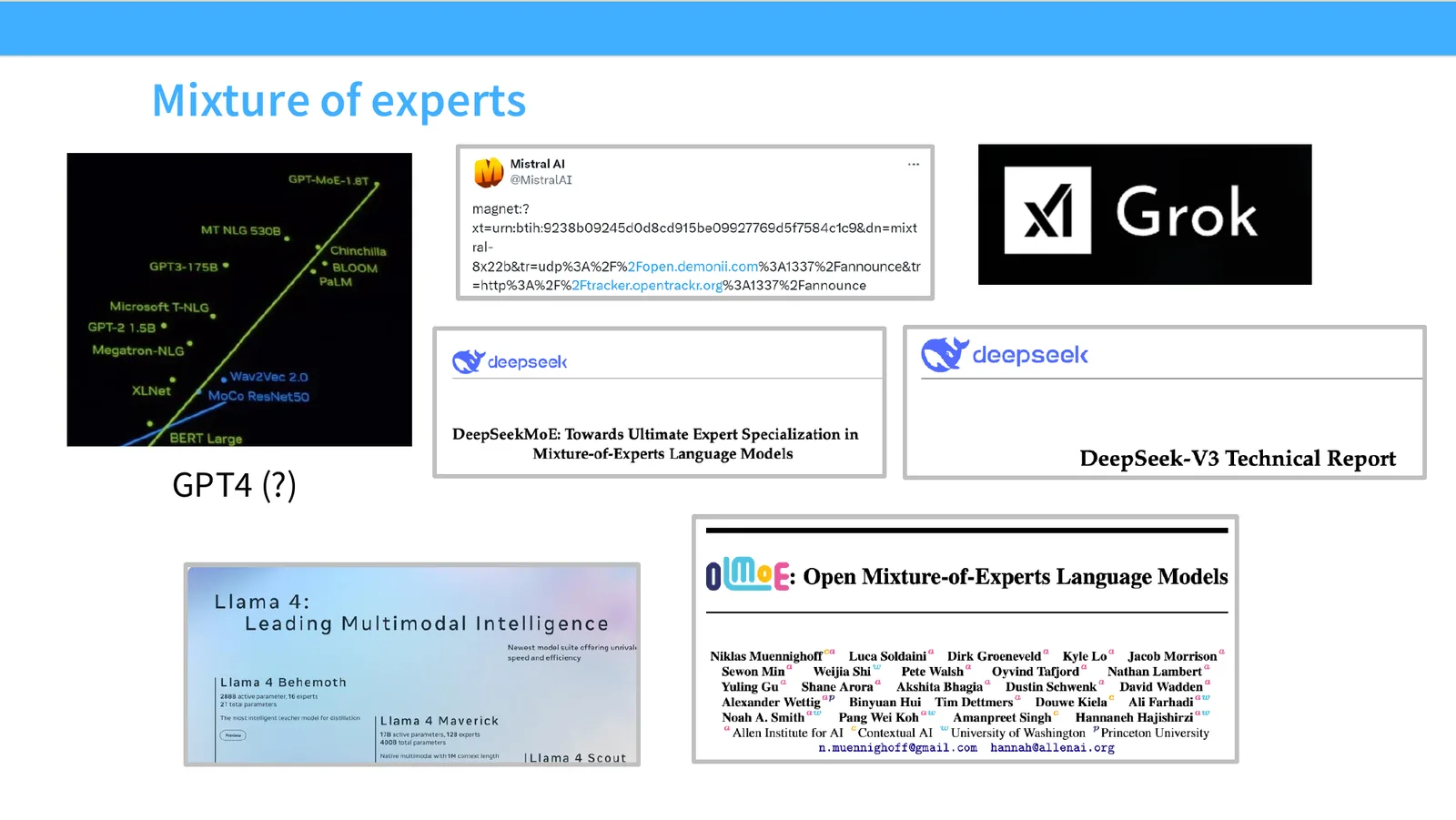
34:15 It might be possible one day to not have any trade-offs, but I think thus far that's where the trade-offs are showing up. Cool. Okay, so now I'm going to talk about mixture of experts. And I think mixture of experts are important to talk about. Conceptually, they don't really change the game. Like one way of thinking about mixture of experts is they are just a more efficient MLP, right? Like you take your MLP and somehow someone gives you just a more efficient MLP. That is kind of what mixture of experts is. But I think you need to understand what mixture of experts is, I think for two reasons. #

34:47 One is kind of this slide of like everyone's doing MOEs these days. Everyone's shipping MOEs these days. You should understand what it is if you're going to want to be people who deeply understand language models and how they work, right? So that's one reason. The other reason is that MOEs actually have some really interesting sort of mechanical components to them. Like if you look at how MOEs are built and what primitives they use, you will kind of quickly see MOE like primitives in many places. And you'll kind of realize, wow, I can do more interesting things with neural networks. So there's a broader reason why I think MOEs are interesting and cool and you should learn about them. Okay, so what is an MOE, right? #

35:29 MOEs are very simple things in some ways. They're just replacements of your MLP. So on the left is your usual MLP for a transformer, right? You've got your attention, you've got some normalization, and then you've got a feed forward, right? Right after that. This is kind of where a lot of the dense, big information processing happens. Now, what I can do instead is let's say I take my big FFN and I'm going to cut them up into smaller FFNs, right? So I now have four feed forward networks. And let's say actually, let's say I don't cut them up into smaller pieces. #

36:00 Let's say they're the same size as my original FFN. And somehow, right, by some magic, I have a system that tells me which FFN to pick for every input, right? Now what I've done is I have 4x the parameters, or at least for my FFN, right? I have four FFNs worth of parameters. But on any forward or backward pass, right, I'm only going to pay one FFN worth of cost, right? That's great. So in some sense, you know, the original motivations for MOEs, if you read the original papers, have this like very parameter-centric view. You know, if you start something like, well, let's say you just wanted more parameters because you believe more parameters are good. Okay, good. #

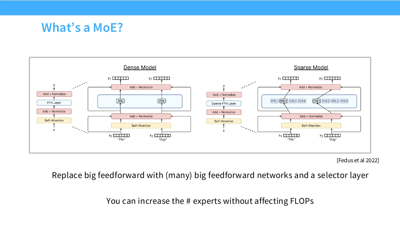
36:40 If we want more parameters and we don't want to pay the cost for more parameters, you need something like something on the right, right? So this is the mental model that you should have for MOEs, right? You want to increase parameters without affecting your flops. #

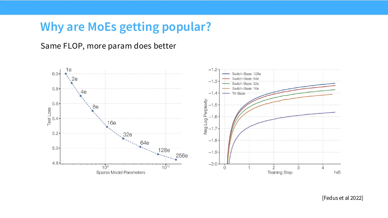
36:54 Now, why are they so popular, right? Every model that you get on Hugging Face or whatever these days are MOEs past a certain size, right? Past a certain size, everything that you get seems to be an MOE. And the reason is because it seems to be the case that for whatever reason, if you keep the total compute the same, but you just increase the number of sparse parameters, right? Somehow the models are generally getting better, right? So this is evidence maybe in favor of the view that more parameters are in fact generally good, even if only a subset of them are active at a time. And I'm going to, you know, refer to some of the original Google papers extensively throughout this lecture. This one's from Fedus et al. in 2022, where they were doing, I think, the switch transformer for this one. #

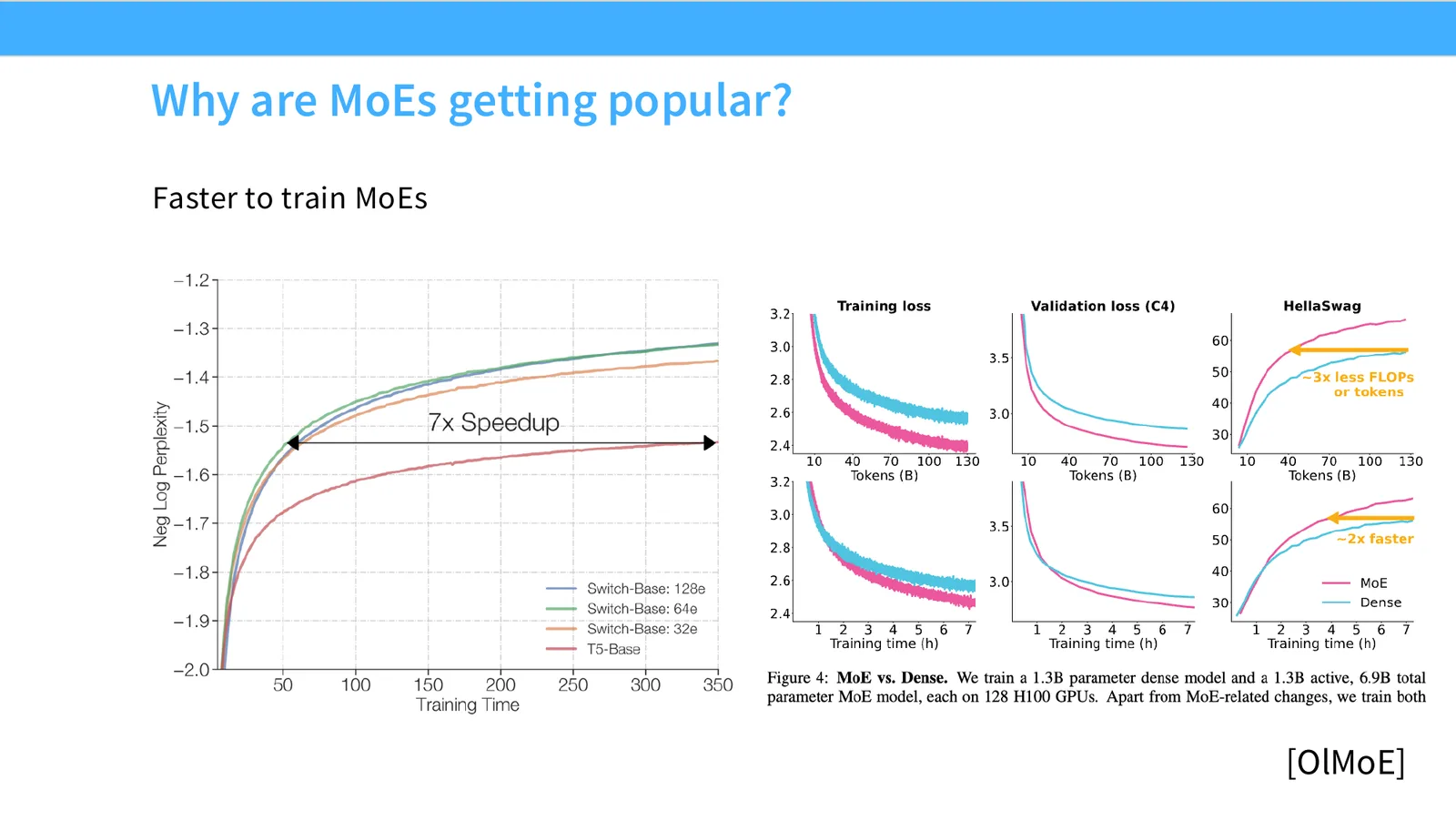
37:41 You know, they're showing, oh, as you increase the number of experts, right? So this is active parameter stays the same, number of experts increases, you know, your test loss for language modeling is just decreasing, decreasing, decreasing. That's lovely if all you care about is your forward pass flaws. On the right, you see sort of similar things as you, you know, you train faster, right? As you increase your training compute on the x-axis, if you have more experts for the same amount of training compute, you just get better performance, right? So for both training and inference, MOEs just give you a free win, right? This is pretty wonderful. It's pretty great. #

38:17 And this is really, you know, something that's been seen many times. This is the same plot from before on the left from the Fedus paper. Last year, I think, AIQ folks put out this Olmo paper, which was their like open source mixture of experts analysis and sort of training paper. And they see the same thing as well. If you look at training loss or validation loss or sort of downstream benchmark performance, you see that in training time, right, these models are doing much better as MOEs compared to their dense counterparts. So something like two times faster or something like that, training MOE relative to a dense model. So you can really see the benefits of sparsity here. #

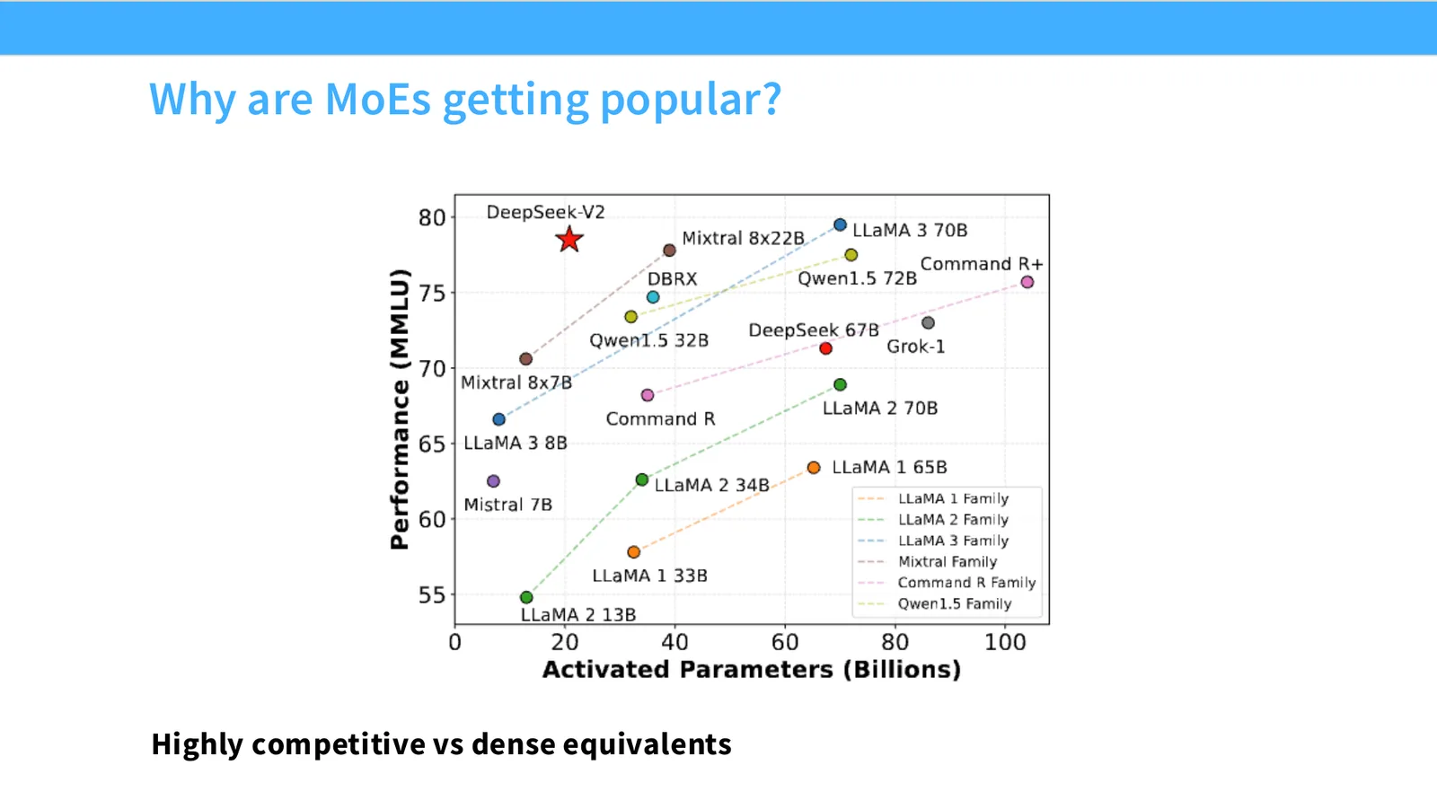
39:02 And, you know, I think the proof is in the pudding. But if you look at all the MOEs that got released, you know, they are much stronger than dense models in terms of activated parameters, which is what matters if you care about inference flops. Or really even, you know, just in general, the cost to train and serve these systems, right? Like the all-in cost. So when DeepSeq V2 and like the earlier DeepSeq MOEs came out, you know, it was really kind of a big shift from a lot of these dense models that everyone else was training. You kind of saw that, wow, we have much fewer active parameters, you know, just as good if not better MMOU performance compared to everyone else. So this is some really good stuff happening with MOEs. Good. Okay. #

39:43 So hopefully I've convinced you that MOEs are like an interesting thing that you should like spend your time thinking about and studying. Oh, right. And then one last thing that I'll say for why this is important is MOEs give you another axis of parallelization. We'll talk about parallelization and systems in three, three more lectures, I think. But parallelization is actually one of the really big important things in LLMs. LLMs are very big, they don't fit in single devices, either to train or inference. So you want many different ways of cutting up your model to efficiently serve or train them. Mixture of experts have this additional nice thing that you can do where your experts within each FFN naturally come in different, you know, chunks, right? Each expert is a natural chunk. #

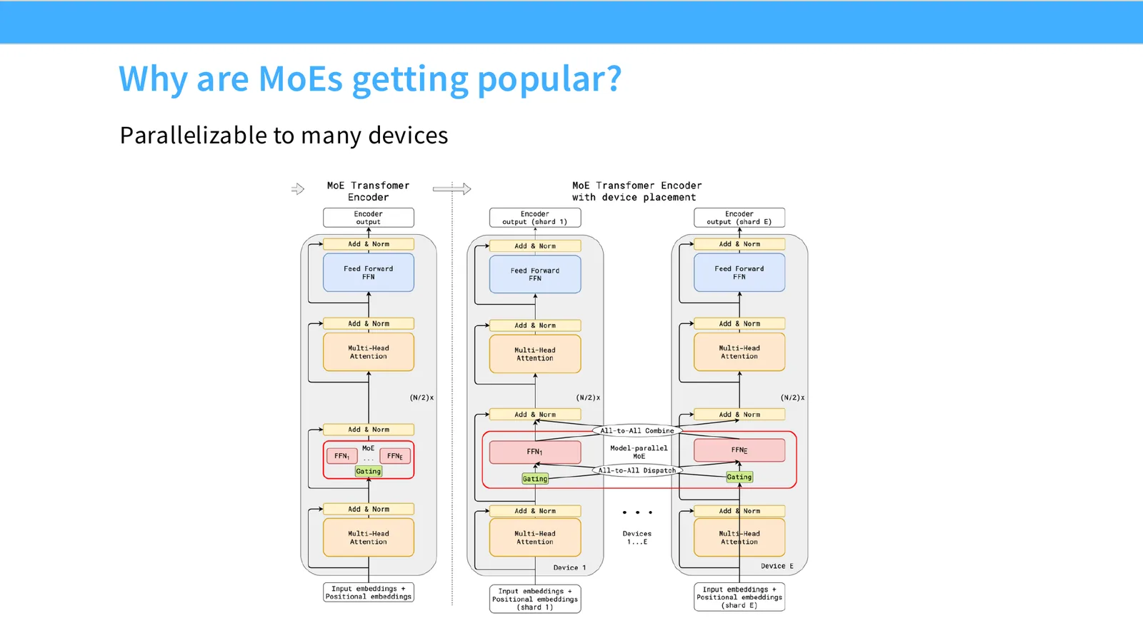
40:26 You can put them on different devices and then you can route the activations to different devices. We'll talk about expert parallel later, which is what this is. But this gives you an additional systems thing that you can optimize, which is very helpful if you want to sort of optimize your server. Okay. In the West, you know, I think there's been several open source releases that are big, strong MOEs. #

08 MoE 战绩：东西方模型对比

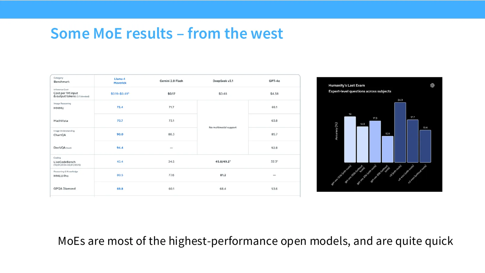
40:49 On the big model side, there was LLMA4 and GPT-OSS from OpenAI. Unfortunately, I guess, open source model releases in the West have kind of stalled for the most part. So there aren't quite as many being released now. But, you know, there's at least two good examples of this. You know, both top tier models in their own right. #

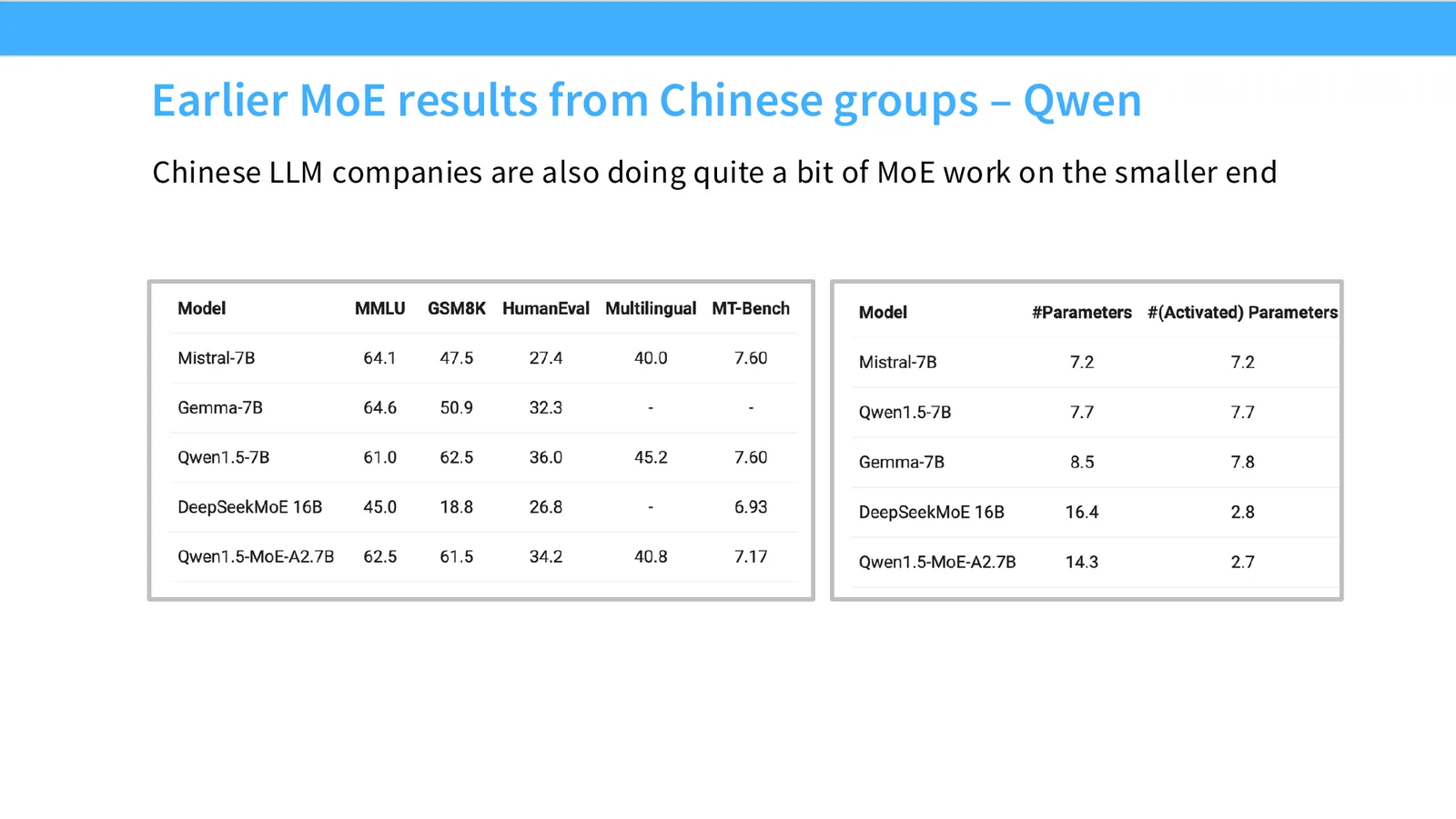
41:11 But I think a lot of the action for both MOE research and training has happened in China. #

41:19 Quen and DeepSeq and some others like MiniCPM did some of the earliest work kind of training and popularizing MOEs. They continue to do really great work on MOEs. You know, if you look at some of the early Quen MOE models, this was Quen 1.5 MOE. You know, they showed that their like small 2.7 billion parameter active model, you know, was doing better than many of the 7B models at the time. And I think some of this early proof of work from DeepSeq and Quen really convinced everyone else in the open source community that this was the right way to go. And speaking of DeepSeq, oh, was there a question? Yes. #

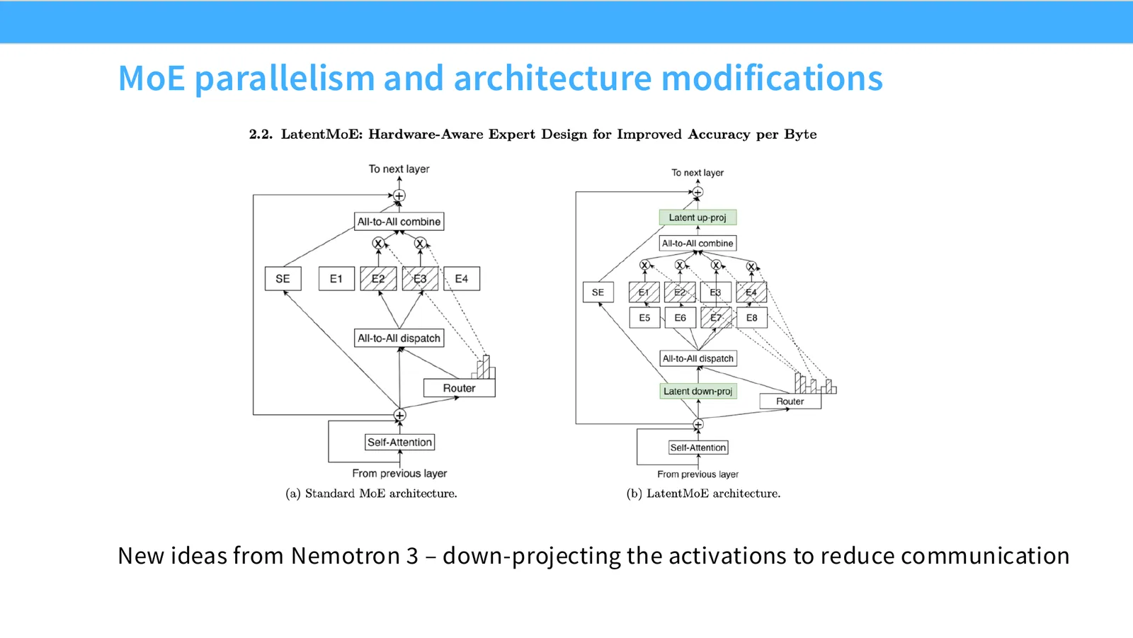
41:57 I guess one question I had about like the expert parallel. Like, isn't there like a communication bottleneck that's built up because these experts are communicating with each other? Yes. So in some sense, you pay the communication cost of like shipping and activation over. And, you know, I will not explain, but I will show you one trick of like how you reduce that. But in general, you're like trading certain things off. You're getting more aggregate flops. You're reducing your memory use. In exchange, you're going to pay for comms, right? #

42:26 So, you know, it's highly dependent on your topology and all these other things, whether this is going to be a net win. Cool. Oh, yeah. During training, the. During, okay, this is the important part. During training, they are also sparse, right? This is really the key thing that makes MOEs hard. I mean, I'm, you know, spoilering sort of the key idea from a few slides down. But it would be very easy if we activated all the experts during training, right? #

42:53 Because then we get to see, oh, which expert is good for my input? So you get to learn how to route. The hard thing about MOEs is that during training, you only have, you know, one or k experts active. So you don't know what happened with the rest of them, right? You only know the ones that activate it. Despite this, you must somehow learn to route, right? So it's kind of got this RL bandit flavor to the problem. But we're not going to solve it with either RL or bandits. We're going to solve it with the power of heuristics and deep learning magic, right? #

43:19 Okay, yes? What is the granularity of switching between experts? So the granularity, as in like the scale at which we route experts at token level. I don't know if, okay, good, good. That was the question. Yes, at the token level. So every token gets an expert. And the routers, you know, just to get your sort of like mental model correct, the routers are super naive, right? They're like a single matrix multiply between your input and your whatever. #

43:41 And so you're not going to do anything complicated. You don't know it's like a medical question or not. You're like, oh, this is a token that looks like it's in, you know, I don't know, Japanese. Let's route it to expert seven, right? Yes? Yes. So is there an upper limit to paralyzing these MOE models in training or in search? Yeah, in general, there's upper limit to paralyzation because, you know, as you shard over more and more devices, the communication cost explodes, right? You will, well, if we get the assignment two design done correctly, you will have to deal with some of these in your assignment. #

44:15 We will ask you to figure out the networking topology and things like this that will make sharding make sense or it's the reverse. Given a networking topology, you'll have to figure out how to shard models and things like this. Yeah. Good. Okay. #

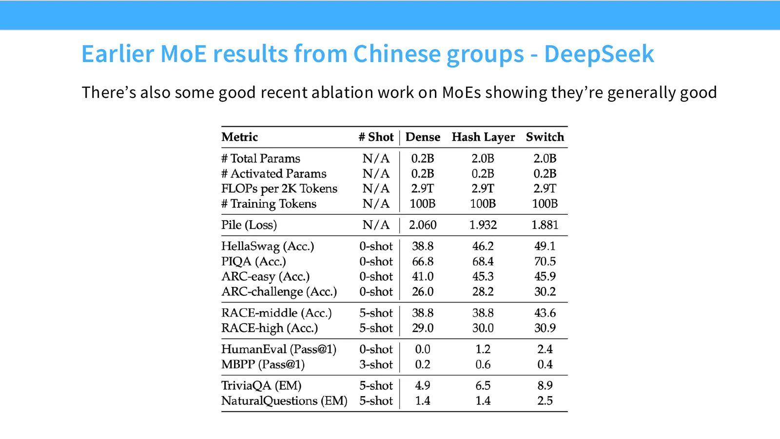
44:29 Right. DeepSeq, you know, now known for like DeepSeq R1 and so on. But I think the thing I really like about DeepSeq, and originally this lecture was a, you know, let's just go through a DeepSeq paper lecture the very first iteration, is that they've done actually really good architecture and LLM science work for a long time. And DeepSeq were one of the earlier ones, you know, going through and showing why MOEs are good and they have a lot of ton of good ablation work on like, oh, what happens if we use a dense layer? What if we use hash routing? What if we use a switch router? You know, all these different kinds of design decisions you can see in some of their earlier DeepSeq MOE papers. So if you're interested in a lot of these questions like architecture design and so on, I would suggest you read our earlier DeepSeq papers. There's a lot to learn from all of these, right? #

45:13 And of course, progress hasn't stopped. #

09 为什么 MoE 没有更早普及

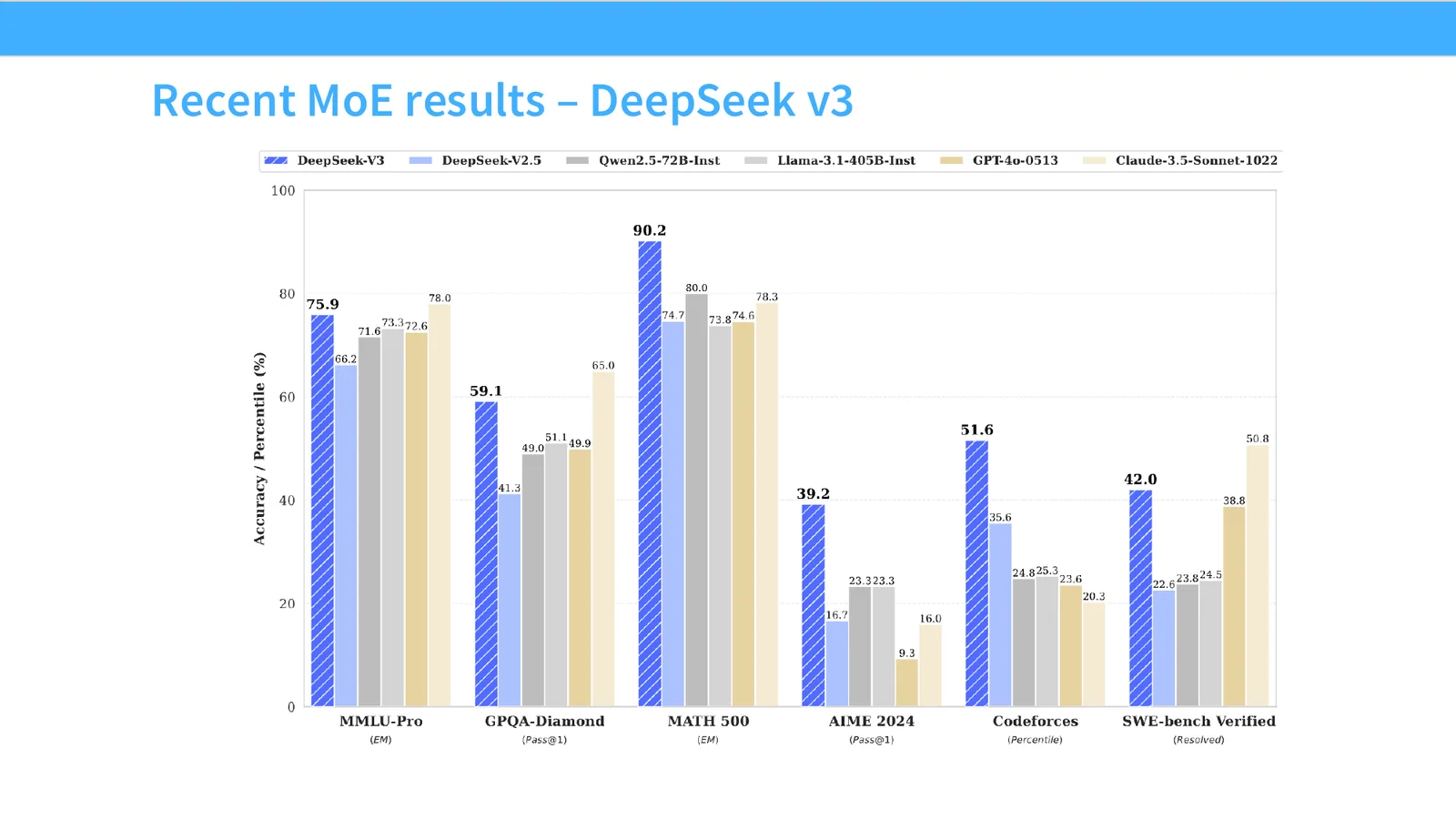
45:15 You know, DeepSeq V3 and V3.2 and like GLM and so on have built these like wonderful, very strong MOE models. It's quite clear that this is kind of where the future of these big models are going to be for the foreseeable future. At least the next couple of years, I imagine, will be MOEs. Okay, so now the question is why haven't they been more popular? In many different ways. I feel like MOEs caught on pretty slowly. You know, you look at some of these papers like in 2022, right? Google was studying and really trying to like push MOEs. #

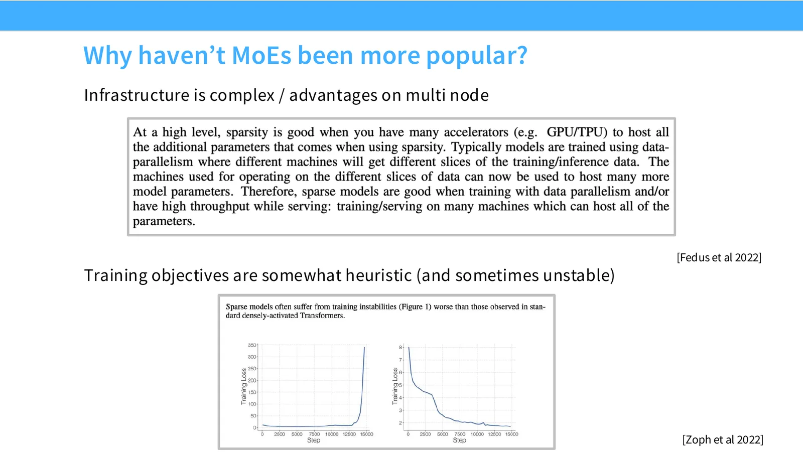
45:51 But, you know, it's only in like 2024 onwards that MOEs really started to catch on. Like why? Also, you know, if you're doing LM research of various kinds, you're probably mostly working with dense models. Like why not MOE models if they're so nice, right? We can save on compute. There's a lot of complexities that come from MOEs. Like it's not easy to train at MOE or to use at MOE or to do many things. You know, the infrastructure is very complex. I mean, there were a couple of questions about parallelization. #

46:19 But this is like generally right. It's hard to parallelize, you know, experts in ways that are like efficient in utilization. MOEs have a lot of parameters. It's hard to fit them on a single device. And if you're training them, the MOEs can really blow up on you. And you'll see why in a few slides why MOEs are just really hard to deal with. But they're just not easy objects to work with, right? I mean, there's good rules of thumb now, but it's not easy. Okay, I'll briefly mention with one slide that there are people that also, you know, kind of mixture of experts, the attention block in transformers. #

10 MoE 结构与路由函数概览

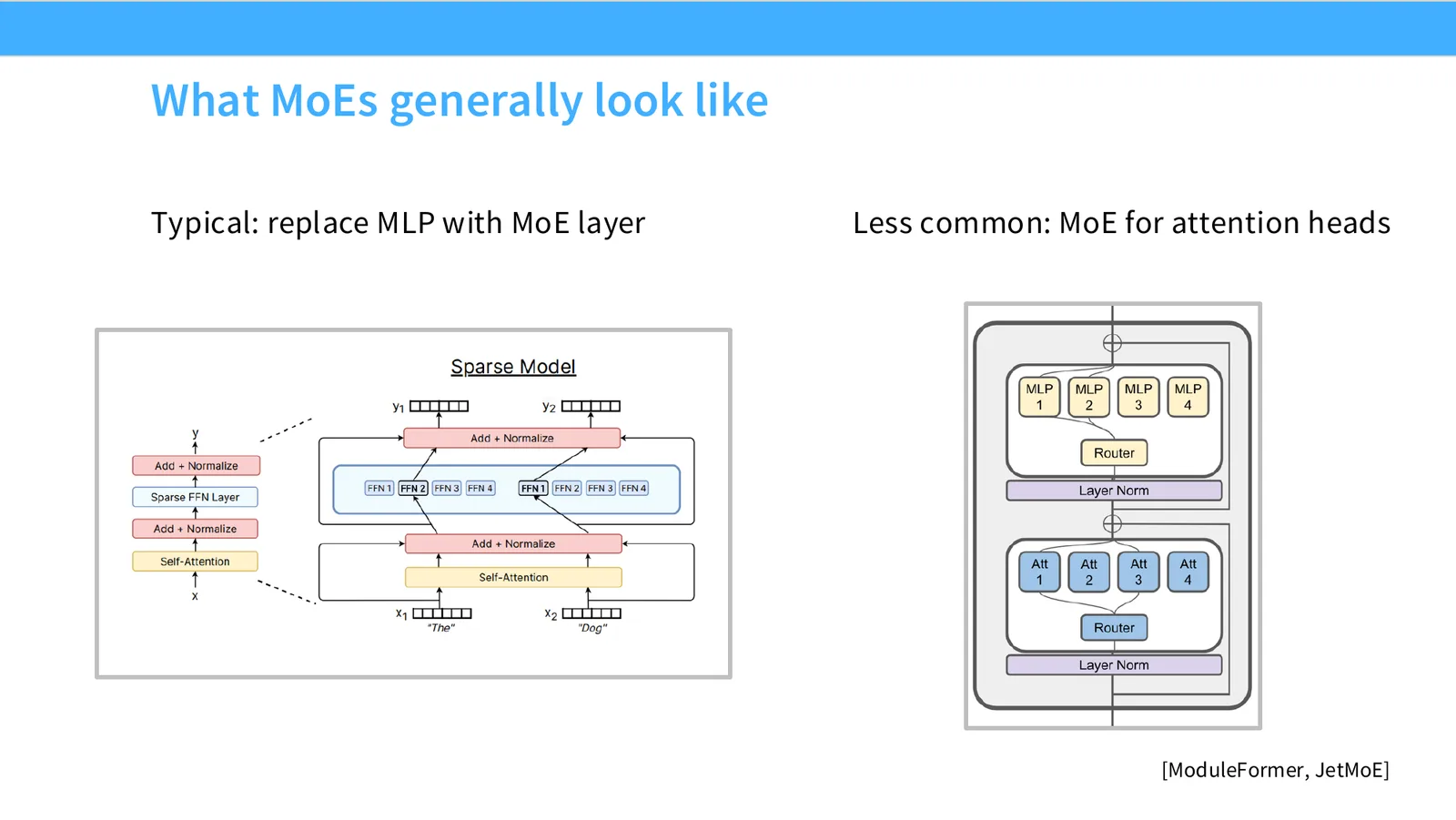
46:54 There have been a couple papers, but they are much less common. And I think the, you know, things that I have seen is that they haven't been quite as easy to tame or to get to work compared to just replacing the FFN or the MLP layer, right? So I'm only going to talk about the left. This is basically what all the big models do. People are not, for the most part, sharding or sorry, splitting up attention heads into experts. #

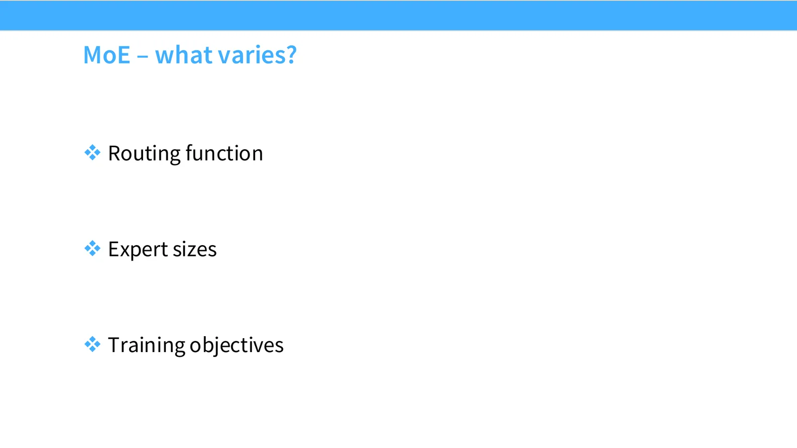
47:23 Okay, so that was kind of the broad industrial overview of like MOEs and like what the state of things are. But now let's like talk about how you design an MOE, how you think about an MOE. So to do that, I'm going to talk about three different kind of axes of variation, right? So what kinds of things can change for MOEs? Well, you can change the routing function, right? We know that MOEs have this core thing of like a router has to send tokens to experts, right? So we can change that. We can change the sizes of the different experts, right? For a given budget, you might have more experts with fewer parameters or fewer experts with more parameters. #

48:01 And then finally, we're going to talk about training, right? Because training is going to be really difficult. Like once you start to realize how MOEs work, you realize, wow, it is not easy to train something that routes tokens to different places. #

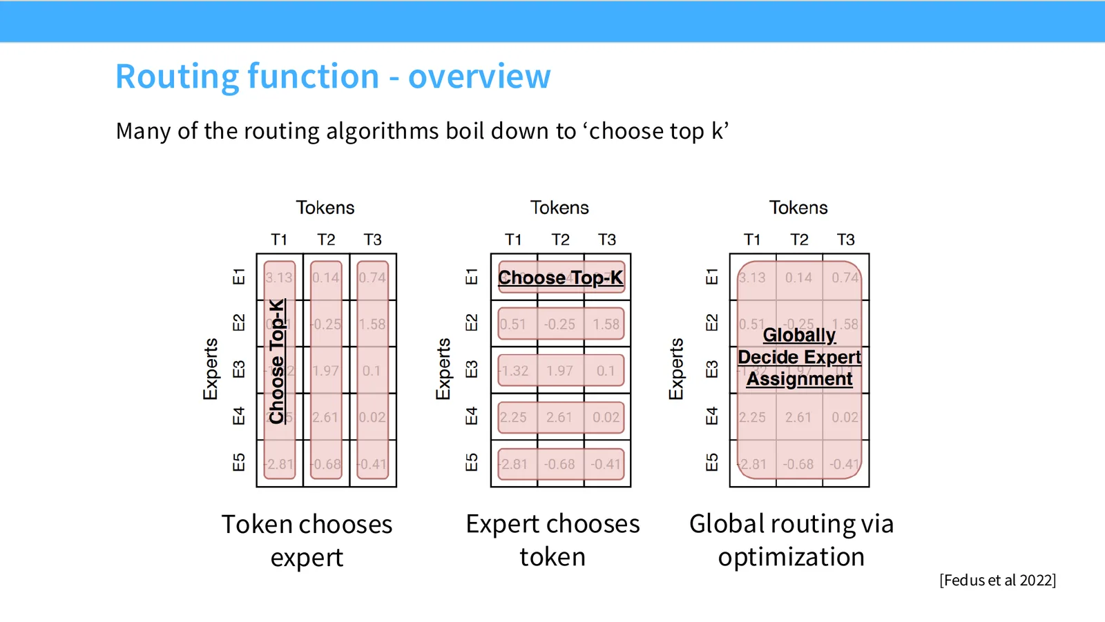
48:15 Okay, so in all cases, we don't want to activate all the experts, right? Like we want to only have some subset of experts active. And so we are going to always be choosing some top K. There is different kinds of choices that you can do. You can have the token choose the expert. You can have the expert choose the token. So each expert picks, you know, their favorite tokens. Or you can have each token pick their favorite experts. Or you can somehow have this like very complicated router that like globally decides, oh yes, you token should go to this expert and this other token should go to the other experts to try to like globally optimize assignments. #

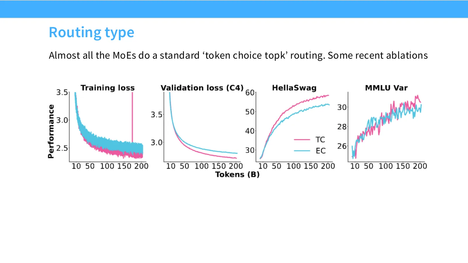
48:56 So basically, almost all the MOEs do token choice top K. And so the token is going to be the one to choose the experts. And there's going to be K different experts that get sort of selected to be in the pool. And you can sort of see, you know, this is from the Olmo paper, differences between token choice and expert choice. You see that token choice is going to get, you know, lower validation losses, higher downstream benchmark scores compared to expert choice. There have been successful expert choice models. I mean, this also trains fine, you know. But token choice has generally been much easier to get working. It has been kind of the standard for all of the models that kind of we see today. #

49:36 I think one of the Lama 4 models was maybe expert choice. But I don't think that's necessarily a strong vote of confidence. #

49:45 What? I don't think, I think that was one of the unreleased Lama 4 models, you know, in my defense. Okay, so I think there's many different ways that you can do routing. So one of the ways that you can do routing is you can actually have a small, small sort of, like a linear projection that says, okay, I'm going to get my input. My router is going to compute an inner product. Each expert has sort of a vector direction and the sort of closest inner product space will get selected. This is by far the most common router. It's used in the classic switch transformer, the G Shard. Those two are the early Google papers. #

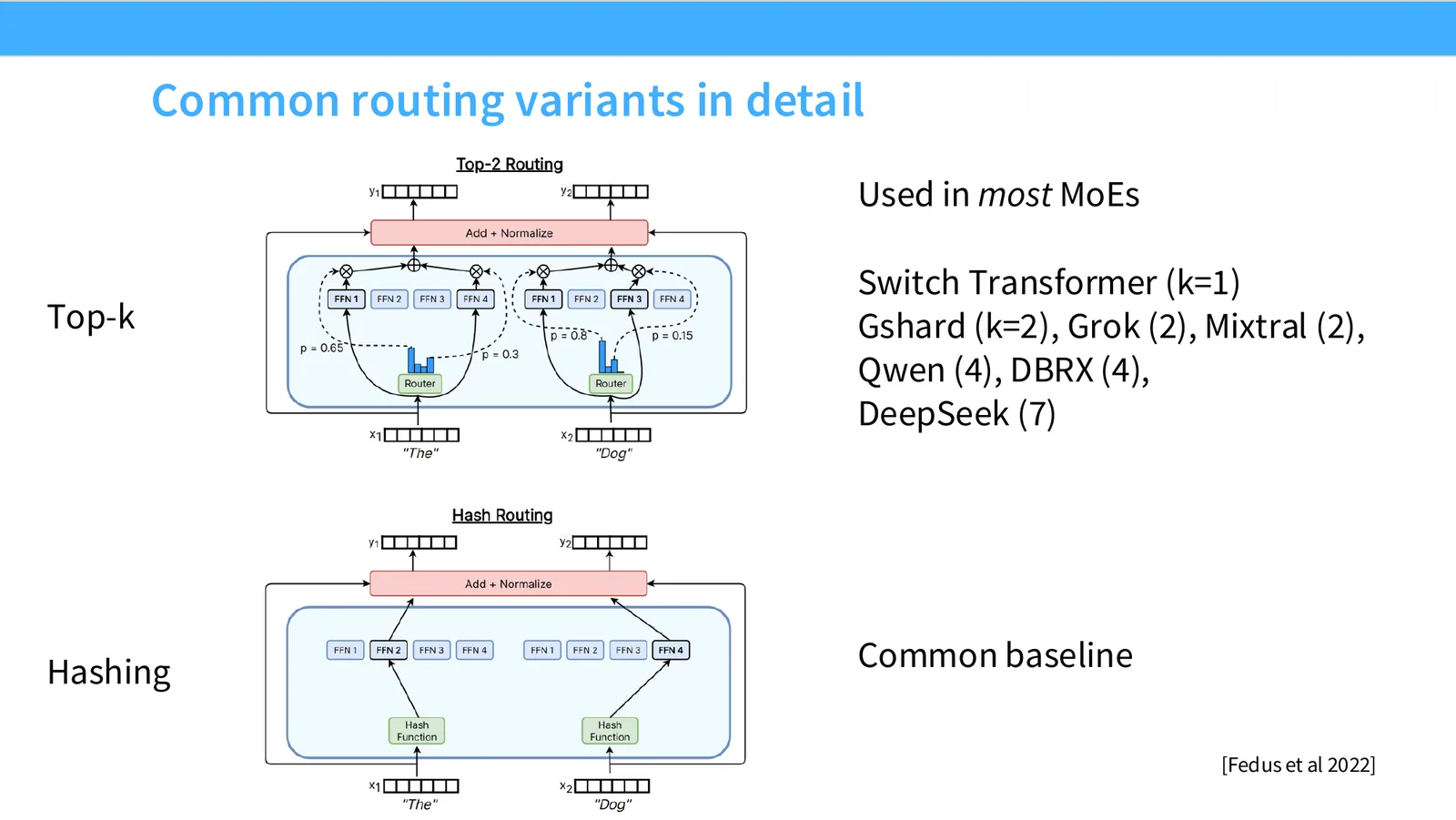
50:21 It's used in Grok, Mixtroquen, DBRX, DeepSeq, and others, right? The number of K that you choose varies depending on, you know, which paper you're looking at. But for the most part, you know, you're just taking inner products. One thing that has always been a little bit serious to me is that many, many papers have shown that actually you don't need to do any sort of like learned routing. You can just take your X's, you can hash them and send them to different feed forward networks. And actually, this is fine too. This sometimes, or this gives gains. Not as much as top K, but somehow hashing based expert routing is also, you know, something that people do. Common baseline in papers, not used in deployment for real reasons, for many reasons. #

51:05 You can do RL to learn the routes. You can basically have a router that's an inner product router. And you can sort of use reinforcement learning to try to treat this router as a kind of policy and then learn it. You know, if you're a machine learning, like classic, you know, learning theory type oriented person, I think this should be the natural way to think about the problem, right? You're like, okay, what am I doing? It's kind of like a bandit problem. I'm selecting one out of K or K out of N. And I don't observe all of them. This is a bandit problem. #

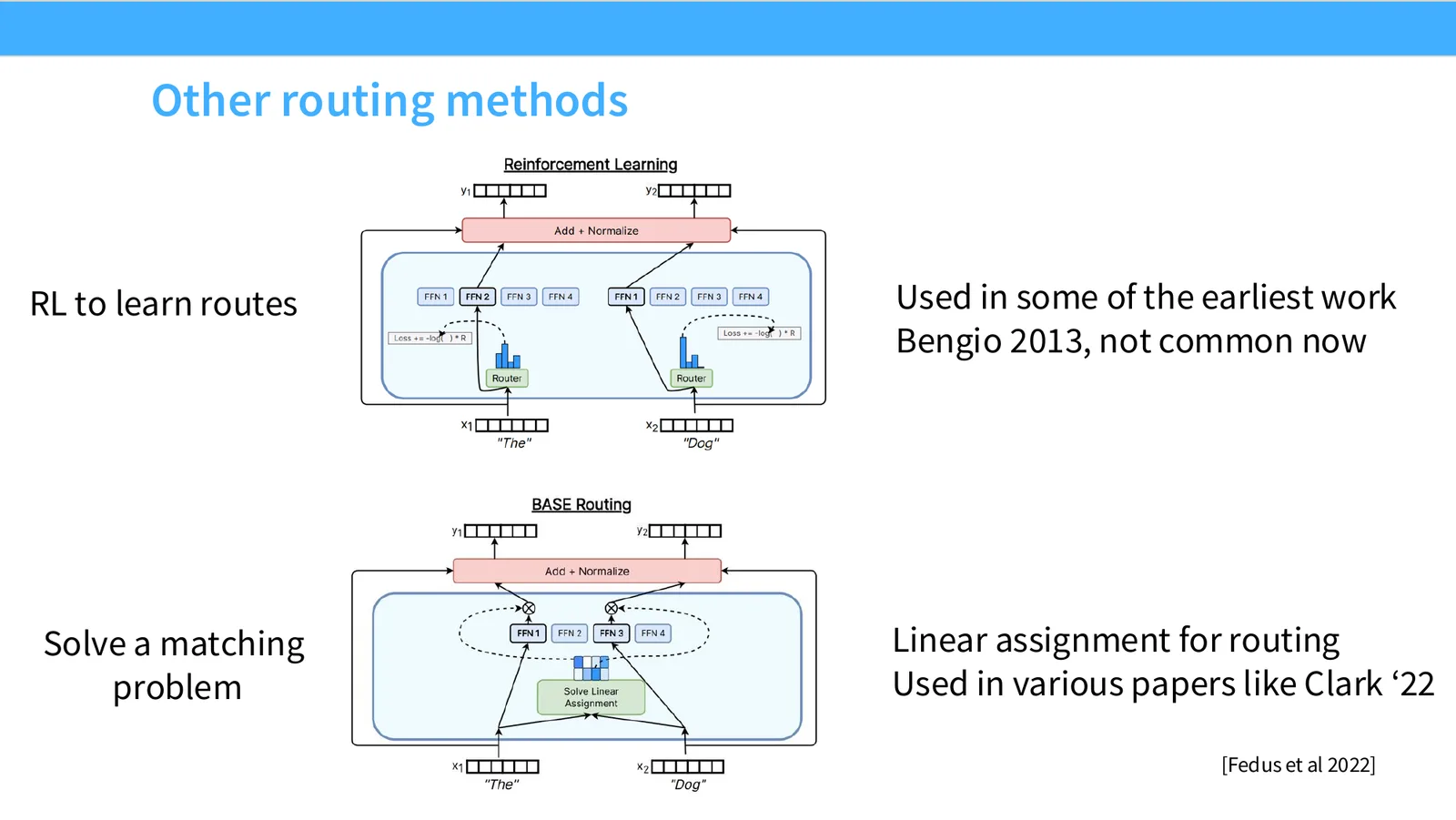
51:36 I will use a bandit or an RL algorithm, right? Used in some of the earliest work, because this is kind of the natural way to think about the problem, like Benjiu in 2013. But it is not a common approach. And I think the reason why it's not common is because, you know, the approaches needed to do RL introduce a lot of overhead in terms of both the RL algorithm and the stochasticity. #

52:00 And what people have figured out is there is a good set of heuristics, like these recipes that you can apply to this very simple classic top K routing scheme that basically just has it working, right? And so there's no reason to do something much more complicated. I will finally sort of mention, you know, an idea that I think is really cool and that I love as a person that likes things that make sense. You can solve a linear assignment problem where you say, okay, I'm going to globally compute kind of the score that says like, oh, it would be this good for this token to go to that expert, right? So you compute this all pairwise scores of how good the assignments are, and you can use linear assignment to exactly solve for the optimal assignment from experts to tokens. It's been used. It's been shown to do good things in some cases. Hasn't been seen at scale at all. I would think because it's, you know, extremely expensive relative to the others to get working. #

52:56 Okay. So top key routing, as I said, is basically the consensus routing mechanism. How does this work? It's very, very simple. And if you, you know, were paying attention in the DSA slide, this looks a lot like DSA, right? You will also notice this if you were reading some other papers like HNets or these other kinds of things. This will appear in many different places. So this is a good kind of pattern to be able to sort of recognize. So what you're doing is you are going to take in your inputs, and you're going to take it through sort of a feed forward. #

53:31 And then I'm going to compute some sort of scores. And the scores that I'm going to compute is going to be the softmax between the experts and sort of my inputs, U. And then this S is going to be the scores. And I'm going to select the top K of those guys. And that's going to be the gate that's going to control each of my experts, right? So this is like input. This is the residual term. This is the FFN. I've got gates. #

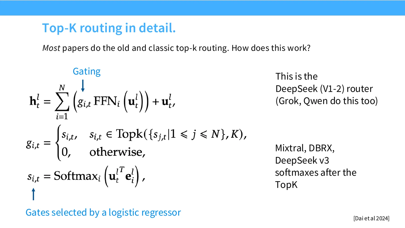
53:56 And the gates are controlled top K, right? This is kind of the equation form of what you would imagine of a top K router. And the only, you know, detail that you're probably learning here is how do I learn my gates? My gates are just learned by taking inner products between a weight for each expert and the inputs that I have, right? Very, very lightweight, right? So there's nothing complicated about the ways that I'm going to select my gates. #

54:20 Even within this simple thing, there's been some innovation and variation from DeepSeq and friends. DeepSeq MOE pioneered this idea, which is now very widely used, called shared experts. This is a very intuitive idea where, you know, in the classic top K router, you would have, you know, K different, sorry, in this case, N different experts. And these experts, you know, you would select amongst them. But sometimes you might say, well, there's some processing, some very common processing that I want to apply to all tokens, right? Like maybe you don't want experts to be different every time. You want some experts to always be applied and then some other experts to be applied conditionally, right? So what DeepSeq MOE did was they took sort of the original expert design. They cut up the experts into smaller, finer grained chunks. #

55:13 And some subset of those fine grained experts were sort of set as shared experts that are always on, right? So these sort of bypass the router. They always process our inputs and they sort of go back on the outputs. Oops, sorry. #

55:27 And this is a nice idea because it turned out that, you know, if you have this classic expert design, you were just kind of reusing a lot of these weights to do common modeling. And so you can offload this into the one shared expert, letting these guys specialize even more. And, you know, as I was kind of saying, DeepSeq is really nice in that they do careful ablations in a lot of their papers. And so, you know, they have this very nice ablation where they look at, you know, zero shared experts. And then you have these big experts, 16 routed experts. And this is really the old G-shard Google design. Compared to, you know, they have very fine-grained segmentation of experts and one shared expert amongst these. And, you know, as you make the experts smaller and smaller and you have one shared expert, you see significant gains from both of those interventions. And for some of these, you know, the shared expert has very significant improvements. #

56:18 Like trivia, QA, natural questions, this blue to yellow gap, right, is shared experts or not. So more experts, shared experts, all generally seem to help. And if you want sort of more validation of these claims and ideas, you see this from ULMO as well. ULMO is, I think, the nice Western sort of carefully controlled MOE study. They do things like, oh, do shared experts help? They conclude that shared experts don't help very much. And, you know, number of experts, they show, you know, doing fine-grained many experts is helpful. So they disagree a little bit on the shared expert point. But, you know, they also have very nice carefully controlled ablations. #

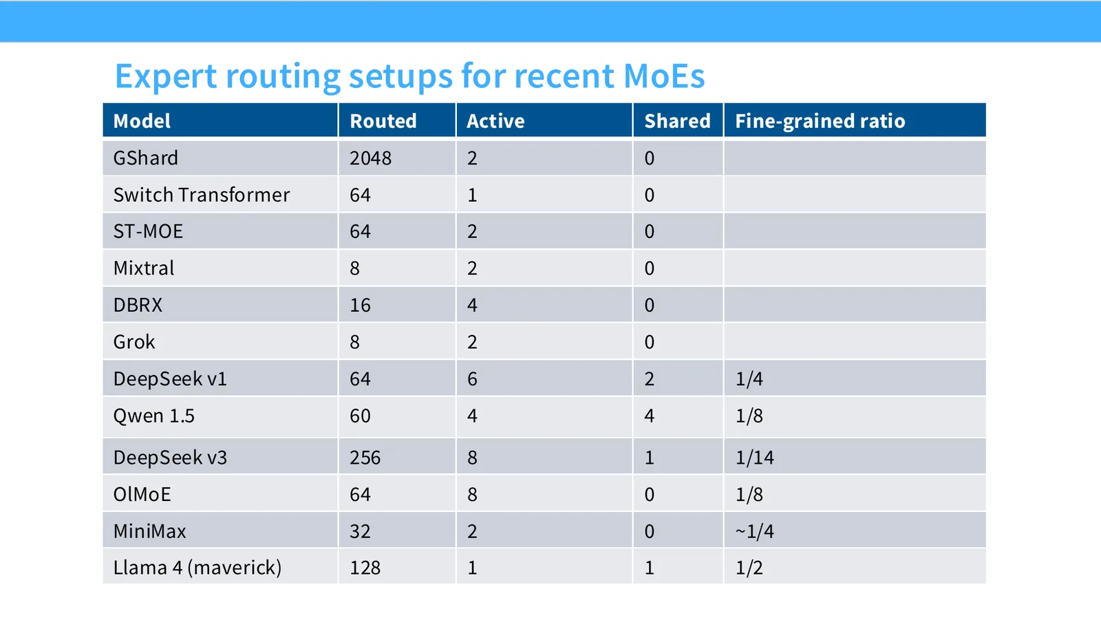
57:00 Many of the recent MOEs do follow essentially the DeepSeq design. You know, there were a couple of early MOEs up until this point. The first three, you know, I keep giving Google praise for doing lots of interesting things. #

11 细粒度专家 + 共享专家与消融

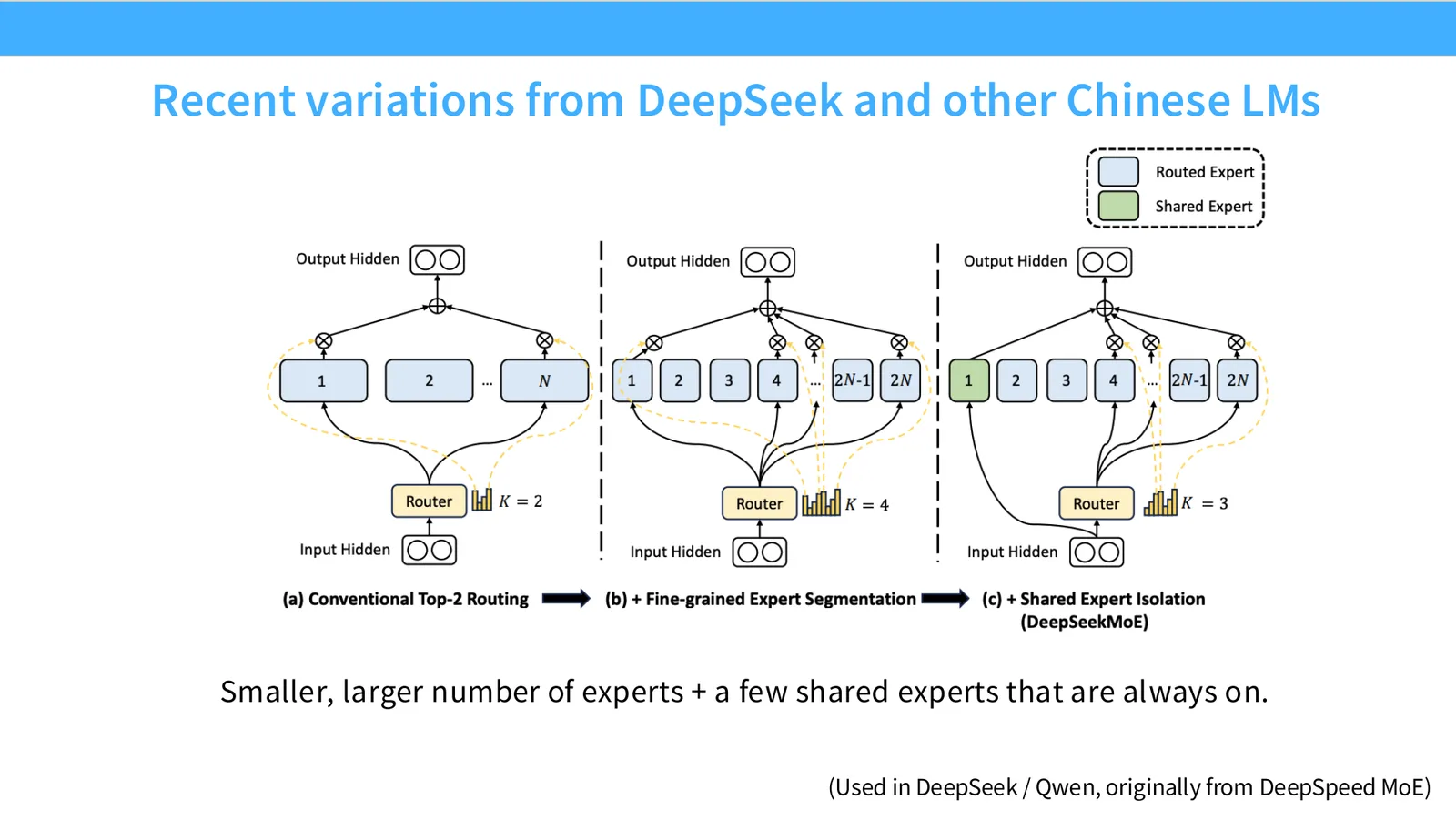
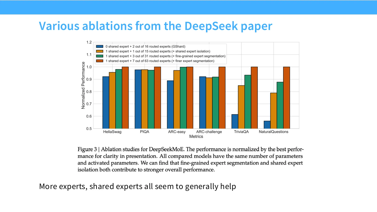
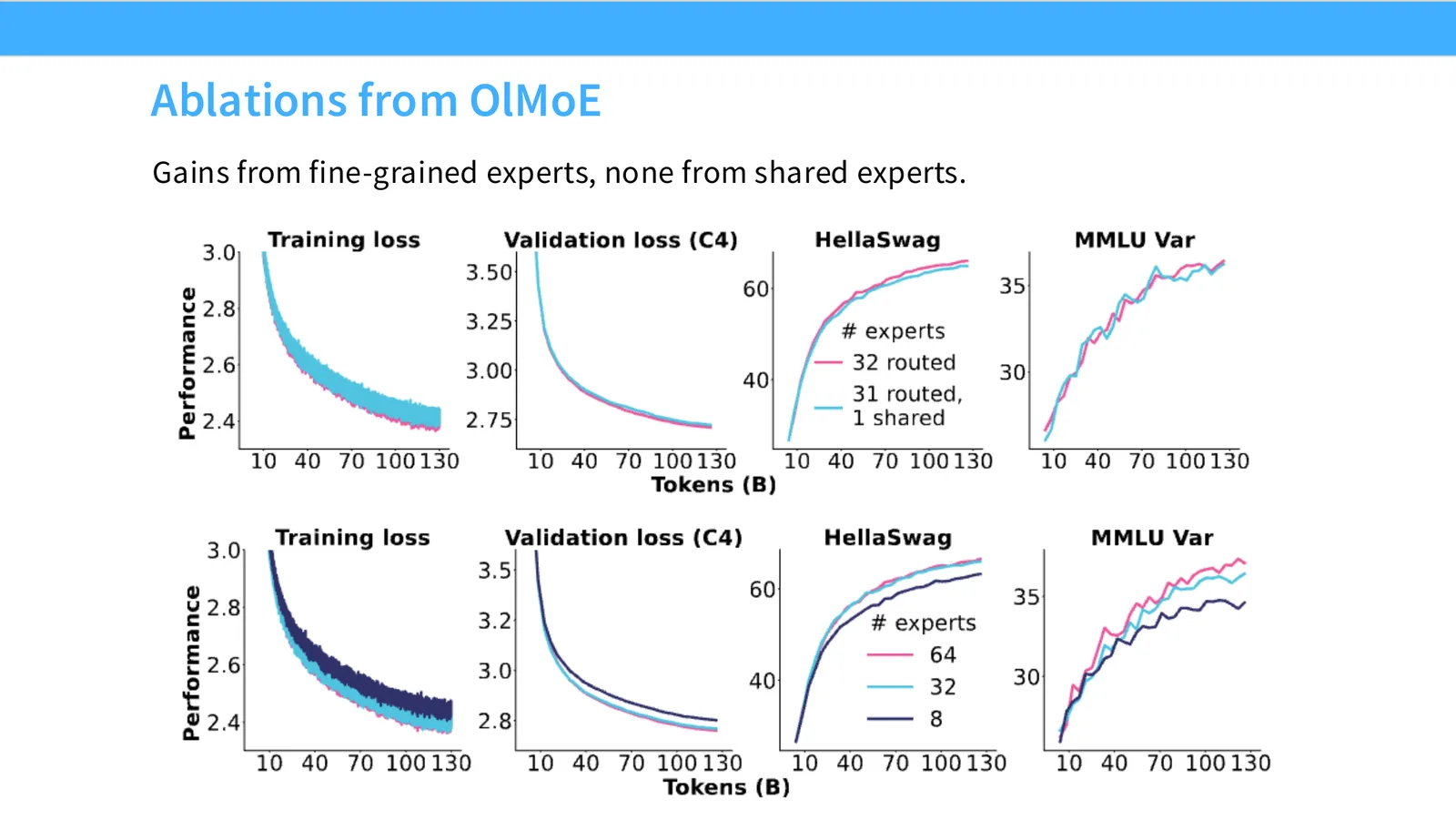
57:15 You know, the first three were from Google. Mixtrel, DBRX, and Grok were some of the early MOE attempts in the West. DeepSeq V1 comes up with sort of both the fine-grained and shared expert design. And then that sort of catches on and everyone else sort of, you know, follows from DeepSeq. I mean, it's a similar, I would say, phenomenon to the LAMA design for dense transformers being, you know, essentially the standard. DeepSeq MOE and DeepSeq V3 are kind of a standard design that people have copied for the MOE side of things. And if you look at like QEN 3.5 or GLM or any of these modern models, you continue to see both shared experts and fine-grained experts in widespread use amongst all of these people. And so that's been a very battle-tested design. #

57:59 Okay, any questions? Oh, yes, good. If there is a shared expert or there are like few shared experts, right? How would parallelization work in that case? Yeah, so in the shared expert case, you know, you wouldn't get any parallelization savings. Like every activation has to route through those. Like you can copy the shared expert to basically eat memory savings to reduce comms cost. #

58:25 Okay, cool. All right, so that's kind of the sort of design space of routers. Now, I want to talk about training MOEs. And this is like, you know, it gets into really surprising and I would say very deep learning things about this. I think initially when I was learning about MOEs, I thought there's no way that we can train these things well or like reasonably. But it turns out there are lots of, you know, tricks that when combined together, like just really work well and robustly for some reason. #

58:56 So as we'll sort of raise in the previous question, right, we don't want to activate all the experts during training, right? Because if we do that, we're going to pay the full flops cost of all of our experts. #

12 训练 MoE：路由不可微与负载均衡损失

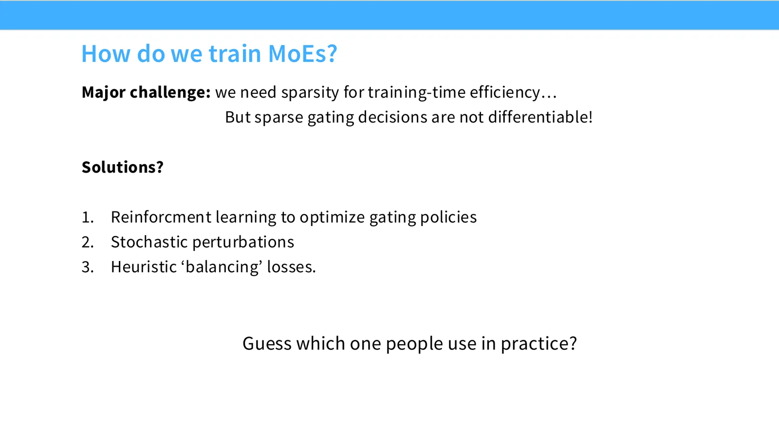
59:04 So in ARC, we have a lot of experts. So we need sparsity for efficiency at training time. But if we have sparsity, then gating decisions are no longer differentiable. And we also don't see all the different counterfactual experts we could have picked, right? So these are both big problems. So there are different solutions. We could use RL to optimize our gating policies. I already mentioned this. Not super popular. #

59:26 You could do things like stochastic perturbations, right? So if you're familiar with like, you know, explore, exploit, bandit style stuff, you could do some of that. Now the third one is you could kind of have a whole bunch of weird heuristics that, you know, deal with the fact that the gating decisions are sparse to balance out which experts go where. You know, guess which one people use in practice. I've been kind of hinting at this. It's number three, right? It's a collection of really interesting heuristics that end up working. I'll talk about the other two first. They're not widely used. #

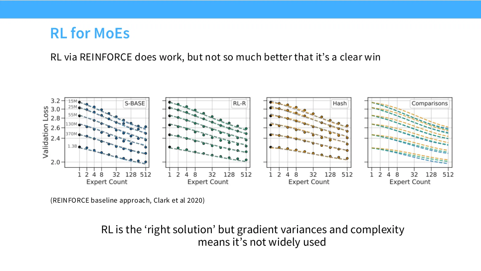
1:00:00 I would, you know, open with that. But I think it's useful to know. So some people have done, you know, this is from Clark 2020, research on things like, can you use RL to learn routers? So it does work. You can use RL, this is the green line over here. That's one of the baseline approaches. It works fine, but because of the gradient variance and complexity, it's not, you know, actually the optimal thing to do. And even sort of some of the approaches that are proposed in this paper, you know, handily be using reinforced gradients for routing decisions. Now, something that's very close to the idea of RL, but sort of starts to move more towards this like heuristic world of like, you know, write down objectives and try things. #

1:00:45 And what I'm going to do is, is this idea of a stochastic approximation. And it comes from the earliest sort of MOE paper from Noam Shadir and others, where what you do is you don't really make a hard decision during training. What you do is you make stochastic decisions. So what you do is, you know, you still have this sort of routing setup. So this H is sort of the, you have the inner product between your parameters and your inputs. This is your, you know, standard routing inner product. But then instead of just doing this, I'm going to inject some noise that's kind of, you know, dependent on the scale of the input. And then that's going to be my H. And now I'm going to keep the top K in softmax, just like I was explaining with top K. #

1:01:29 And then that's going to be, you know, the output that goes in to my top K function. Now, if you look at this, you know, what is this doing? Well, it just means that if you have two experts that are like closely tied or it's like very close to each other, then stochastically you'll pick one of them and not the other. Right? And as you back prop, you're going to back prop in a way that like, you know, the experts that are helpful will get high weights. So this, you know, perturbation allows you to like tie break and explore a little bit more. And hopefully the gradient structure is such that if an expert is helpful, it's going to sort of emphasize the expert more and it will get higher and higher weights in general. Right? So this is one reasonable thing that you can do. #

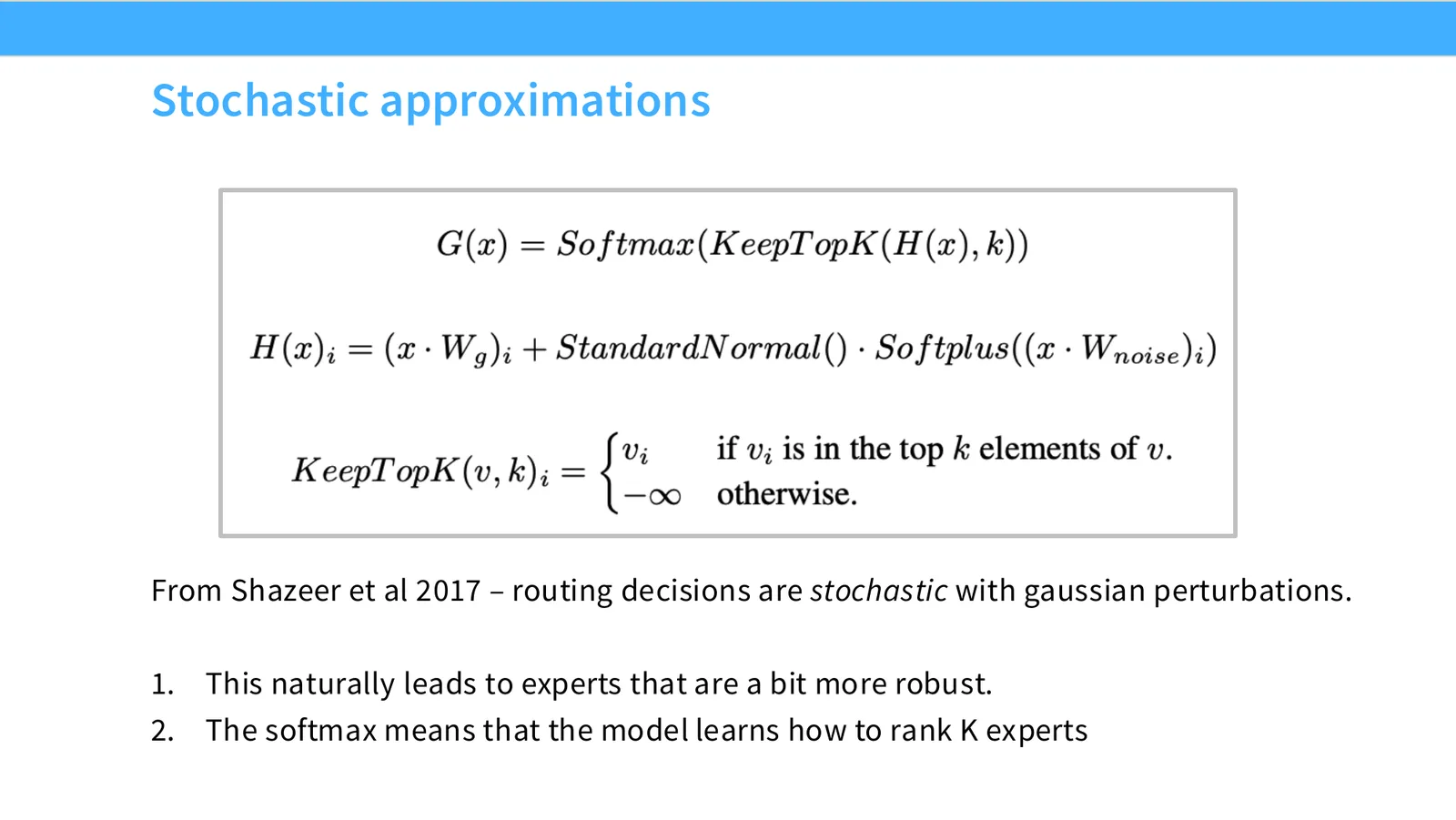
1:02:09 It leads to experts that are a bit more robust. And you, the softmax, you know, allows you to learn how to rank all these K experts, right? Rather than just doing a hard selection of top K, you're kind of weighting by these elements. #

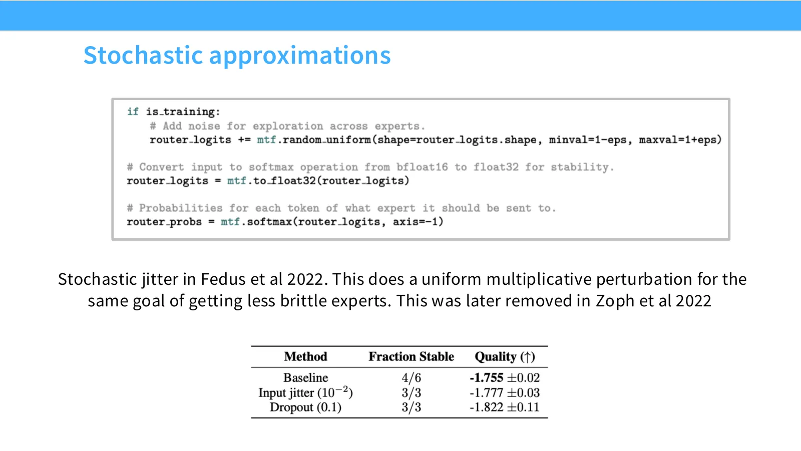
1:02:25 Okay. There's another sort of scheme that's very closely related that's done in Fetis et al. in 2022, which does kind of a uniform multiplicative perturbation. They do this for the reason of like hardening the experts, like making them robust. This was a useful thing to do, but this was later removed in later Google papers that do sort of routing. And it's not really clear that this is, you know, necessary at all. You kind of see later ablation showing that, you know, not doing any, any of these like stochastic sort of robustness tricks actually helps with both stability and overall quality of the final trained MOE. So this kind of suggests, you know, you don't need necessarily the stochastic exploration terms. #

1:03:13 So this takes us to what you actually do, which is a series of sort of heuristics that, you know, in the end is going to give us a working MOE. And a lot of these have to do with essentially balancing. So what's the problem if you just do normal gradient descent, ignoring any of these like exploration exploitation concerns? Well, what's going to happen is you're going to first route to your top K experts. And then sort of the strongest of those experts will get sort of more signal. Your back prop is going to say that expert was good. You know, increase the weight of the expert, right? Move that parameter closer to that. So you get this rich gets richer effect where sort of experts that are chosen get very strong weights. #

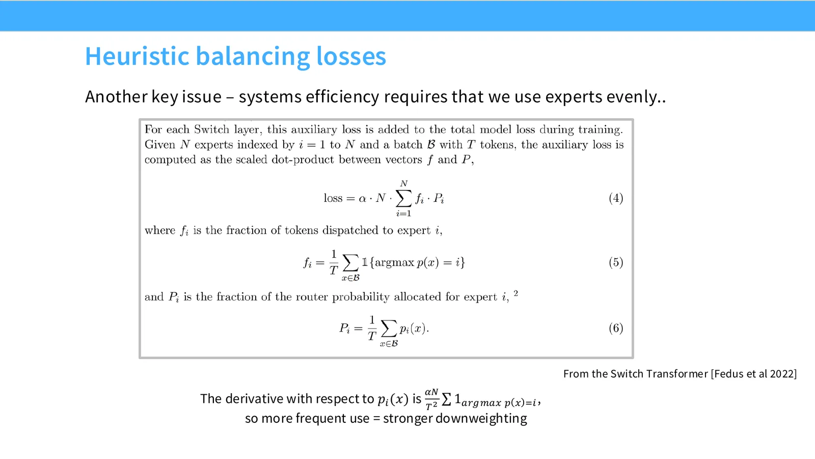
1:03:53 Strong weights means that they're selected more often and they kind of run away taking on everything. And so this expert collapse phenomenon or like expert, you know, starvation phenomenon is a very, very real problem. And in some sense, this is the core issue that you have to solve with sort of heuristic training of MOEs. And so what do you do? Well, what you do is you add a sort of heuristic loss. To the total modeling loss. And this loss is supposed to balance out the tokens that go to different experts. And sort of one approach, which is done in the switch transformer over here. You can kind of look at what this does. #

1:04:31 So this is, you have different experts going from one to n. And you have a batch of tokens. And what you want to do is you want to make sure that these two inner products are kind of small. Okay, so what is happening here? F is the fraction of tokens that are dispatched to any single expert. And then P of I is kind of the softer version. This is not just the whether the token is dispatched to an expert. This is the total probability mass of the router that's allocated. And you multiply these two terms. #

1:05:02 And this is like, at least to me, not a thing where you would derive it from first principles. I think the easiest way to kind of see what this thing is doing is to take the derivative of this object. So if you take the derivative of this with respect to P of I. And P of I, remember, is the probability mass allocated to an expert. Well, the derivative is going to be the fraction of tokens that are allocated. So in some sense, you can think of this as a penalty in the gradient space, where the more tokens you get, the sort of more negative gradient you get, right? So this is trying to push down the probability mass on very popular experts proportional to their fraction. And that's kind of the action of this loss, right? That's the way to think about it. #

13 DeepSeek 的均衡目标与去 LBL 实验

1:05:45 So, you know, the objective itself in equation four might not be clear to start with. But once you sort of reason about the action of the gradient, it becomes kind of clear what this is trying to do, which is to push down popular experts. #

1:05:59 So, you know, then we can actually take these ideas and essentially reconstruct DeepSeq v1 and 2's MOE system. So what do you do to build DeepSeq MOE? Well, you're going to do your normal losses, and you're just going to back prop straight through the experts, ignoring all this non-differentiability and exploration concerns. But you're going to add per expert balancing that's identical to the switch transformer, what I just showed you, right? So you're going to have this loss that multiplies F, which is a fraction, and P, which is the total mass. But, you know, DeepSeq folks, they're very savvy with their sort of systems design. So they don't just balance the experts, right? They also want to balance by device. So if your experts are allocated to some devices, so let's say, you know, my machine over here has four experts. #

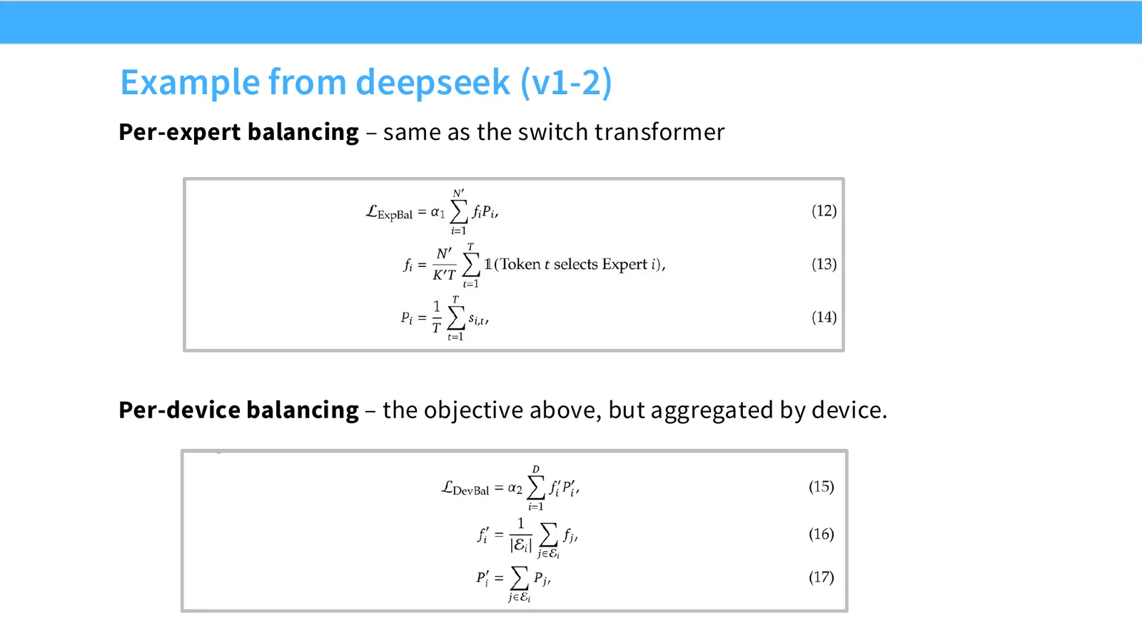
1:06:45 This machine over here has another four experts. You want those two machines to be balanced. So both of them are kind of running at full utilization, right? So you don't want to just make the experts even. You also want to ensure that the devices are even, right? So this is a secondary objective. It acts in exactly the same way. If you look at the function here, instead of experts, you're just operating on each device's fraction. You apply the secondary device balancing loss just for utilization reasons. #

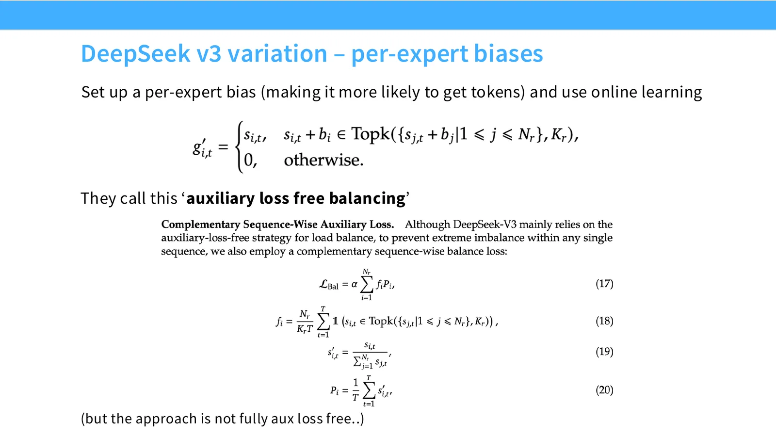
1:07:11 In DeepSeq V3, they have sort of a per-expert bias term that they use. And they use kind of an online learning trick to sort of balance out experts, sort of getting rid of some of these auxiliary losses. But sort of, you know, they do in the end have to add some of these auxiliary losses in order to ensure like extreme imbalances don't happen. So I think, you know, I add this as kind of a side note that, you know, DeepSeq V3 and others have started to get rid of some of these, like, I would say uglier auxiliary losses. But there's no kind of solution that fully gets rid of them so far. #

1:07:51 Okay. The last thing I'll talk about with load balancing losses is, you know, you might ask, like, do I need to deal with this, right? It's all a bunch of complicated heuristics. I wish I could just get rid of the load balancing loss. But if you remove the load balancing loss, you know, kind of the effects are pretty catastrophic. #

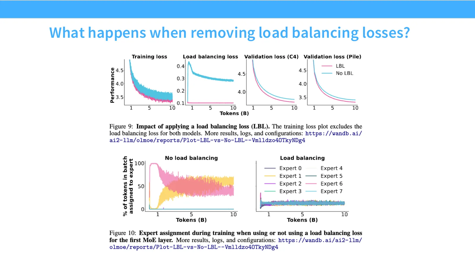
1:08:09 These are both from the Olmo paper where they do this nice ablation of removing the load balancing loss entirely. If you have the load balancing loss, you've got this pink line at the top, very nice normal curves. Remove the load balancing loss. You know, your losses, you know, significantly increase. And your training loss also is not doing so well. Maybe more tellingly, if you look at, you know, which experts are doing what, with load balancing and without load balancing. That's these bottom panels over here. You see a really, really stark difference. Without load balancing, almost all the tokens are going to two experts, right? #

1:08:43 The yellow expert and the pinkish expert that you see here. Whereas if you have the load balancing loss, even though we have this kind of heuristic thing going on, all of these experts are being utilized across the tokens. We have this nice, even utilization, right? So we do kind of see that the load balancing loss does what we expect. And without it, you know, we've thrown away a ton of parameters. Those experts are doing absolutely nothing for most of training, right? So this is kind of how MOEs are trained. And I think, you know, just to go back, this is pretty surprising to me. That you've got this thing that's like kind of non-differentiable. #

1:09:17 You're doing this top case selection. And it is honestly a pretty complicated object. And all you really need to do is to just add this balancing loss to even out the experts. And then the rest of it, you treat it as if you can just pump gradients through the system. And the model trains very nicely. And I think a big part of this is, you know, this dynamic that if an expert is useful, you're going to reinforce it. And that's a sort of positive reinforcement cycle that's nicely sort of balanced out by evening things out, right? Those two dynamics cancel each other out. #

1:09:50 Cool. Oh, and the final thing I'll say is, you know, that same trick is used in DSA, right? We already saw the top-k thing. It's used in things like HNets, if you're familiar with that. That was an attempt to remove tokenizers. And so I think you'll see this trick more often in the future, where this idea of like top-k selection and using load balancing or other kinds of auxiliary losses to enable that non-differentiability will be sort of an ingredient of future architecture design. Yes? #

1:10:30 Yeah, so some papers have a visualization of which tokens are activated by which experts. And because the routers are so simple, it's not like, you know, experts are like smart experts. They're not like medical experts, legal experts, or whatever. You do see that certain tokens are routed to different things. Like, you know, punctuations might be routed to one expert. Or like other symbols might be routed to one expert. You know, non-English language character sets might be routed to another expert. But it's not really something where you can like look at it and be like, oh, this is the Wall Street Journal expert or something, right? Nothing like that. #

1:11:03 There's no semantics in maybe one way. #

1:11:08 Yeah. #

1:11:11 Yeah, the per expert loss in principle, if it's perfectly enforced, will also enforce a per device balancing if your experts are evenly split, right? But I think at least my interpretation of that is, you know, you don't want to crank up the per expert loss so high that you got true full uniformity because that has deleterious effects on training dynamics. But per device is important enough that you're willing to add on a little bit of extra loss to encourage per device balancing over others. #

14 系统侧：并行策略与 MoE 工程

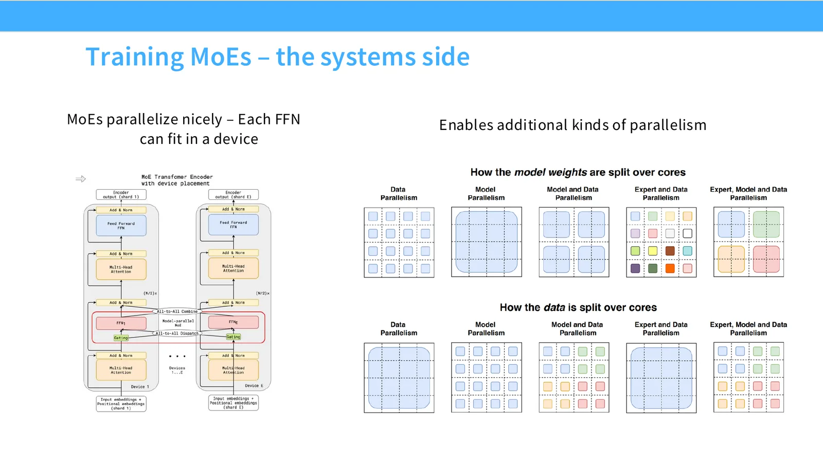
1:11:37 Cool. Okay. So now I'm going to talk a little bit about the system side of things before we wrap up. So training MOEs has additional fun systems dynamics that are introduced. When I talk about parallelism, I'm mostly going to talk about, you know, the standard, let's call it, forms of parallelism. You can, you know, split up your data into many small chunks. Or sorry, you can split up your data over many small chunks. You can take your one data set and split it up over many sort of machines. You can do model parallelism where, you know, you can take your model and maybe you can, you know, split up your model over different machines. #

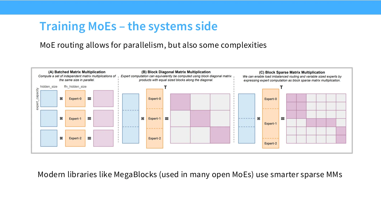
1:12:13 And you can combine those two in various ways. You can, of course, do that. But I think the thing that we realize is each of those parallelism techniques has some sort of limit, right? For data parallelism, you know, you're maxed out your batch size, right? Once you hit your batch size, you can't parallelize by data anymore. For model size, there's natural sort of like cut points where you can cut your model. Once you exhaust those, you can't parallelize anymore. If you combine this with expert parallelism, you get another additional nice axis to parallelize on. And when you do this, a lot of the underlying implementations for this allow you to take advantage of sparse matrix multiply that has been built into GPUs. #

1:12:54 So another thing that I'll mention is like if you're, if you have multiple experts, right? Let's say on one GPU, one way of thinking about it is to say I'm going to have multiple small matrix multiplies. But this is not nice because you ideally want these like bigger matrix multiplies where you can reuse caches and do all sorts of things. So instead, what you can do is you can, you know, nicely leverage sparsity. And block diagonal, of course, is the most basic form. But you can use much more sort of complicated forms of structured sparsity that are sort of natively supported in hardware to allow you to essentially multiply sort of experts and inputs in very, very clean ways very fast. Right? So this is another reason why MOEs are nice. If you think about the sort of computation patterns of MOEs, they almost correspond to these kinds of structured matrix multiplications that are very easy and efficient to support in hardware, right? #

1:13:47 So there's this hardware architecture co-design that's kind of happening with MOEs. #

1:14:18 So this is another reason why MOEs is a very important tool to use a very important tool.! #

1:14:52 drawbacks of having a smaller hidden dimension size, right? So you can actually do these kind of projection tricks to nicely control the trade-off of communication and having your MOEs paralyzed. #

1:15:07 Okay, one final sort of trivia, let's call it detail, of MOEs that I think is fun, but it has been solved in recent years, is stochasticity. If you do MOE sort of infrastructure naively, what you'll find is that unless your experts are sort of perfectly balanced on your input sort of distribution, you'll find that certain experts might be much more popular than others. And if, you know, some expert, like let's say in this case, expert zero is just a really popular expert, you're going to actually start running into situations where this expert sort of queue of tokens just starts building up and building up and building up. And eventually you'll get to a point where you say, my queue is so long I have to start dropping tokens, right? In the earlier generation of MOE inference sort of infrastructure and code, a lot of what happened was you would just actually silently drop this expert and you just proceed on with your computation as if nothing had happened. You know, you just send a zero back and pretend that that was fine. And this means that, you know, you can have like these weird stochasticities where if other users, you know, sent in queries that hit the experts that you're using, then you could actually get a worse result because they would kind of bump you out of the expert queue. You know, these kinds of very strange things happen. But these days they're sort of drop less architectures that have gotten rid of a lot of these issues. #

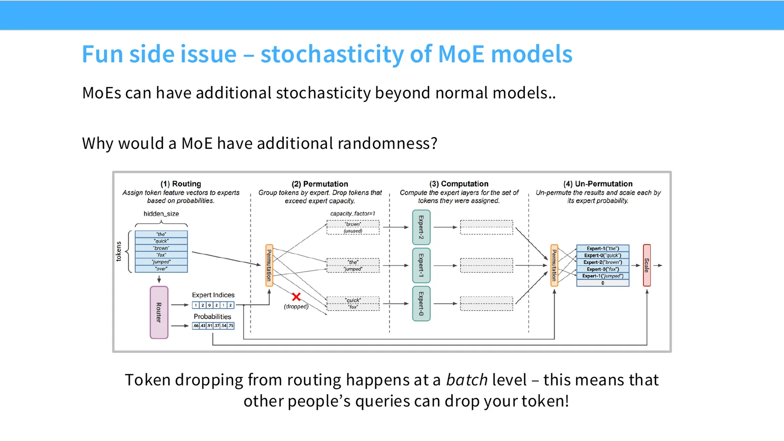
1:16:26 So this is no longer really a issue. So mega blocks and other sort of very common open source MOE frameworks don't have this issue anymore. #

1:16:35 Okay, so the last thing that I'll talk about in terms of the design of MOEs is this issue of stability. We've already talked about stability issues in the context of architecture design last lecture. But, you know, if you remember what I said then, I said, you know, exponentials are bad, divisions are bad, which means soft maxes are, you know, danger zone for stability issues. Now, what have we done with mixture of experts? Well, we have introduced yet another soft max in the routing, right? Because we're going to do top K, we're going to do soft max, and that's going to be sort of how we route to experts. Now, you know, people have long noticed that the soft max operation in MOEs are potentially very, very dangerous. Barrett, Zoth, and others in early days of sort of Google MOE design sort of had an entire paper on MOE stability, and this was one of the things that they noticed. #

15 训练稳定性（z-loss）与微调问题

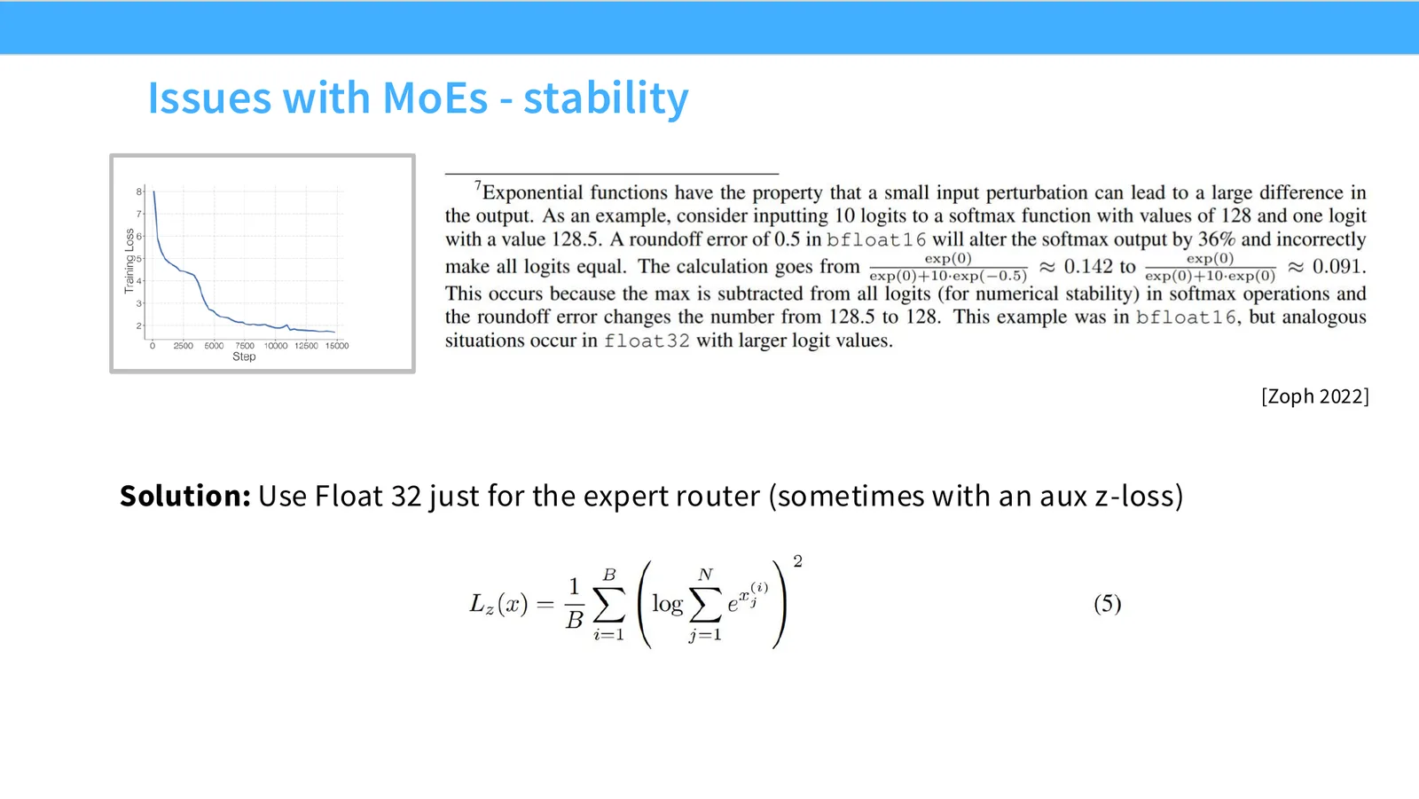
1:17:28 And, you know, I'm going to go into some of the details. You know, you'll see the solution fairly often for some of the more sensitive and tricky parts. You know, you might end up using something like float 32 for just the expert router. You might have a Z loss as well here. We've talked about Z loss before. In order to control the soft max stability issues that we saw. #

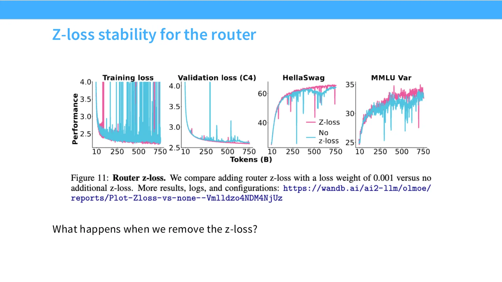
1:17:49 Z loss, I think, was quite popular actually to do MOE router work. MOE router stability even in the early days. ULMO, which I've been talking about extensively, has done ablations on, you know, adding or removing Z loss. You know, it's quite clear from these very spiky training loss curves that Z loss on the router can be quite helpful. #

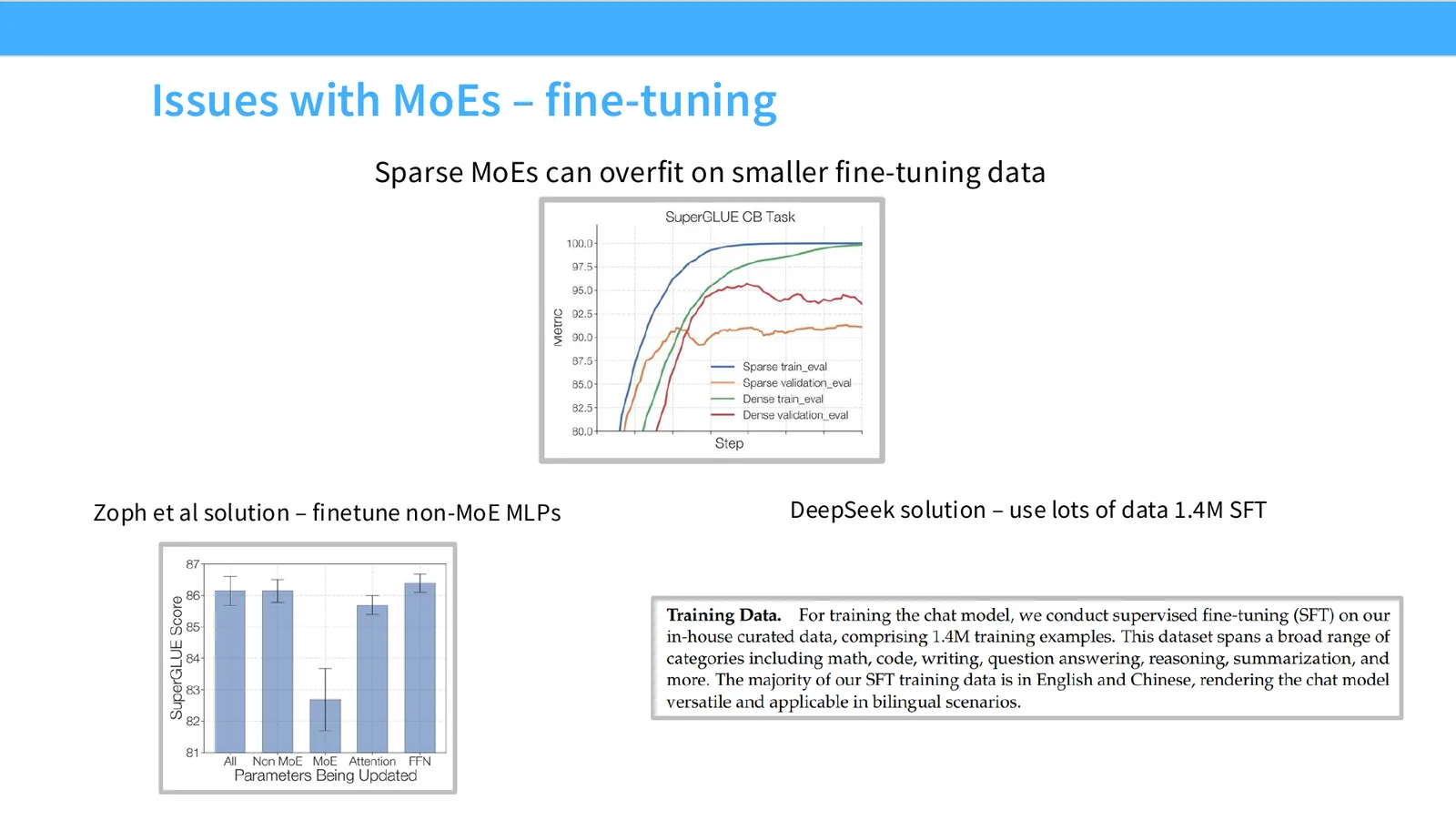
1:18:11 There are other issues with MOEs that you can end up with. And I think, you know, you probably all have experienced this maybe recently if you work with language models. Which is that MOEs can be pretty annoying to fine tune. They have so many parameters that if you're trying to fine tune the experts, you actually end up with very sort of serious overfitting issues. So you can kind of see that if you have your dense models, train and val are, you know, fairly close. They don't overfit crazily. But if you look at the sparse, train and val gap is, you know, extremely large as you fine tune these models for, in this case, downstream tasks. I think it was one of the glue benchmark tasks. Now, you know, you could have a case where, you know, you fine tune non-MOE feed forwards. #

1:18:59 You could also fine tune just the tension. These are pretty common interventions that people do. Especially the attention fine tuning is something that I see quite often with MOE works recently. But if your model has non-MOE layers, then of course you can also just fine tune those. And Barrett-Zoff and others, you know, were kind of arguing for those. And of course there's also the kind of bitter lesson version of this. Which is, you know, maybe you should just use 1.4 million examples instead of, you know, whatever number you have. #

16 Upcycling：从 dense 模型初始化 MoE

1:19:29 If you have a lot of data, you know, you can retrain basically the MOE entirely during your fine tuning stage. And you won't have quite as much of a generalization gap. #

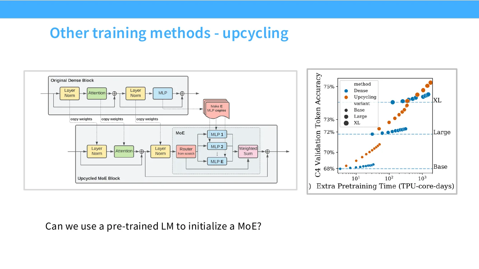
1:19:39 Okay, the last MOE specific trick that I'll mention is this idea of upcycling. This has actually become a lot less popular in the last year. I don't think I've seen a single upcycled model this year. But it's a cool idea. And also there were some very nice models earlier on using this trick. So I kind of want to mention this. So upcycling is this idea that, you know, if you want a MOE, maybe you can just take a dense model that you've trained. And then you can instantiate a MOE based on that dense model. And the idea is you just copy everything, including the MLPs. #

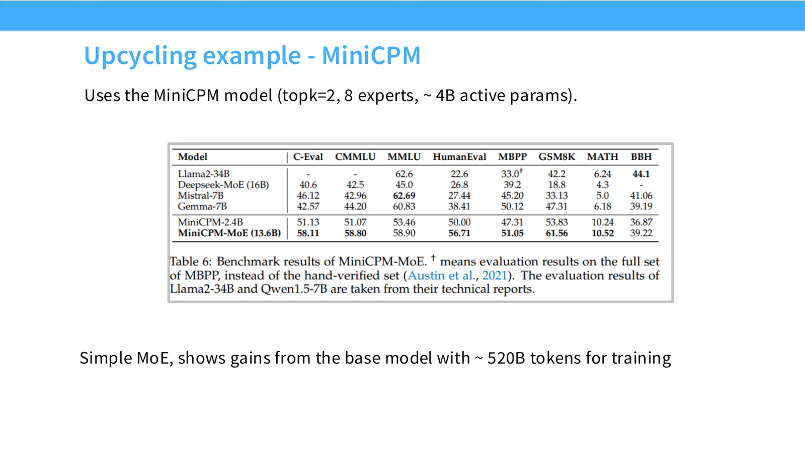
1:20:15 You just make a whole bunch of copies of these MLPs. You have a router which, you know, have a random initialization. And then you just train this model. And if you do this, then, you know, because of the stochasticity of which inputs go to where in the MLP, you're going to get these experts that start to specialize. And in the end, you'll actually end up with MOE. And in sort of some of the earliest papers that proposed upcycling, you know, they showed that an upcycled method could get, you know, much better sort of language modeling sort of value, in this case, accuracy, performance, sort of upcycling a dense model rather than continuing to train the same model, which is kind of a cool thing that you can show. People have sort of validated this kind of at scale in many ways. So mini CPM is another sort of, you know, Chinese model that, you know, I quite like because they do a lot of carefully controlled ablations. They had an MOE where they took their mini CPM 2.4b model, #

1:21:15 they upcycled it to a 13.4b parameter model, and they got a bunch of, you know, almost free wins from doing that. #

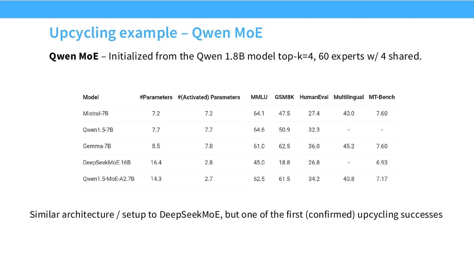
1:21:25 QUEN also, you know, when they did their QUEN MOE, initialized from their 1.8b QUEN model, you know, they upcycled that to a QUEN 1.5a 2.7b model, and they ended up with, you know, one of the first and, you know, one of the very high performance models. It's, I think, one of the first larger scale upcycling successes. Of course, these days, I don't think anyone's really upcycling anymore, because you don't really train dense models and then convert them. You might as well just train your big, you know, hero run on an MOE to start with, right? #

17 DeepSeek MoE v1 → v2 → v3

1:21:59 So I don't think we see this quite as much, but I wanted to mention this, because I think it's an important thing to know in the action space of a mixture of experts models. #

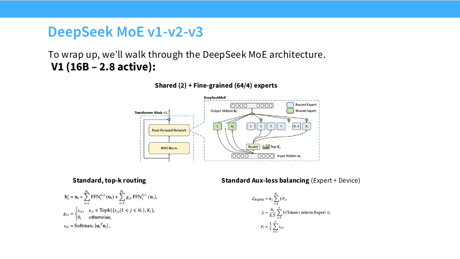
1:22:11 Okay, so the last thing I kind of want to end with is I want to just walk us through the DeepSeq models, V1, V2, and V3. I think there's kind of a lot to learn from the evolution of DeepSeq models. And also, if you're interested just in general about MOEs or architecture design, I would encourage that you read the DeepSeq papers. I think they're very well written. I think they have a lot of details that are worth digging into. So the DeepSeq MOE architecture at V1 is, you know, already actually the prototype of a lot of different modern MOEs. It's got the shared and fine-grained expert structure. It uses standard top-K routing with the auxiliary loss balancing. I mean, in some ways I would say this is like the prototypical, like platonic ideal of a MOE model. #

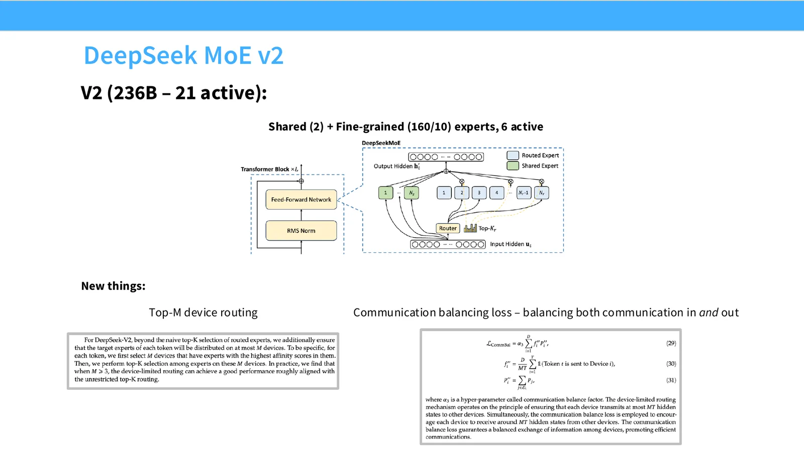
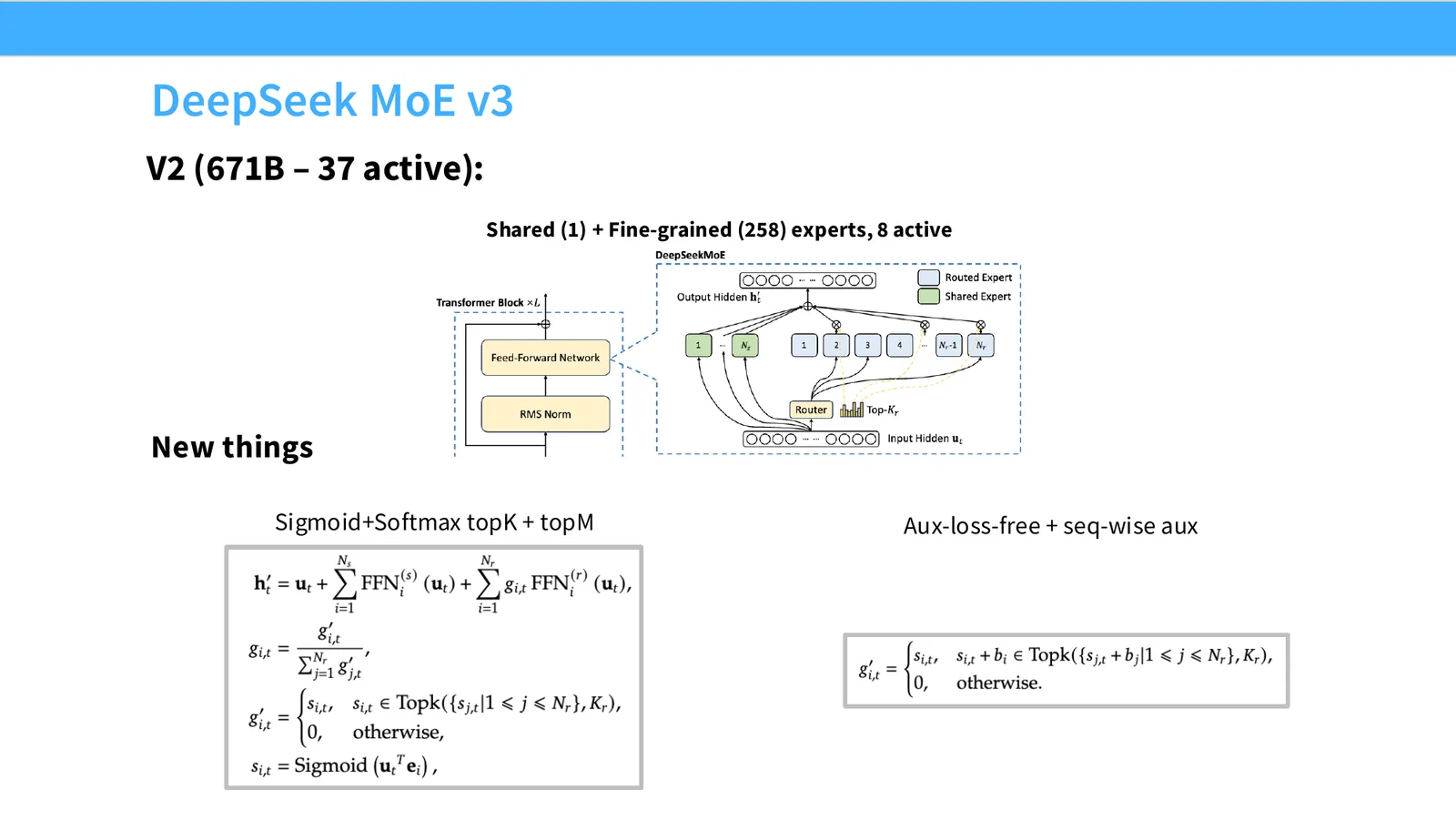
1:22:55 DeepSeq MOE V2 kind of just like scales this guy up, right? So you've got two shared experts, many more fine-grained experts, and you've got this device routing component, and you've got a communication balancing component. Both of these are essentially adding auxiliary losses to optimize systems. I think it's important to realize that, you know, successful language model training is not just about, you know, deep learning. It's also about really respecting your systems, right? So DeepSeq V2 is really a reflection, I think, of this philosophy. And then in DeepSeq MOE V3, you know, they've still got the shared and fine-grained experts design, but they've got sort of different ways of doing balancing. They've got this auxiliary, they've gotten aux loss-free ways of balancing the different experts. And they've sort of switched to using sigmoid plus softmax, which is a different way of sort of weighting their experts. #

1:23:47 But really mostly similar. Finally, since we're already here, we might as well just walk through the rest of DeepSeq MOE V3. #

18 Bonus：MLA 多头潜在注意力与 MTP 多 token 预测

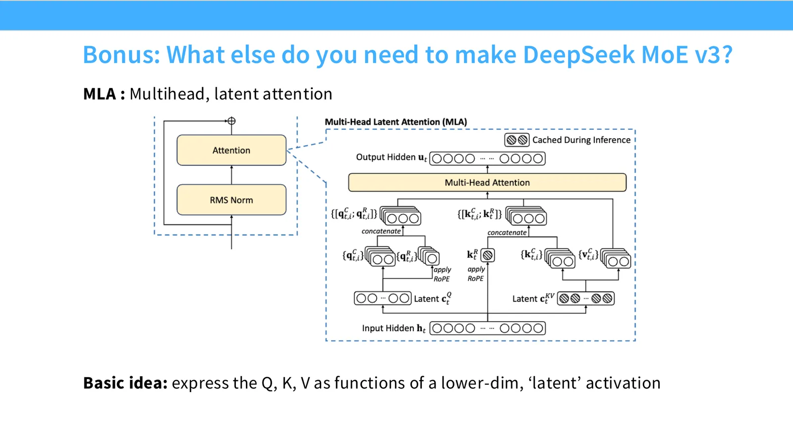
1:23:54 They've got lots of other cool things. I'm a big fan of how they think about systems. They've got multi-head latent attention where, you know, instead of doing QKV sort of directly, what you're going to do is you're going to represent them as this lower dimensional latency. So you have your hidden input. Instead of directly producing your Qs, Ks, and Vs, you're going to first produce the C, and then you're going to produce your QKs and Vs as a function of that. And that allows you to get sort of significantly improved savings. Instead of KV caching all your Ks and Vs, I only need to store these Cs, right? And the Cs are hopefully lower dimensional, right? And that's why it's called MLA, like latent activation, because these Cs, which are latent, are the KV cache quantities that you need to save. #

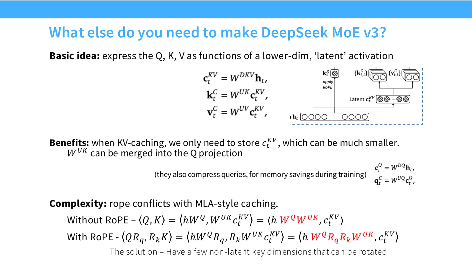
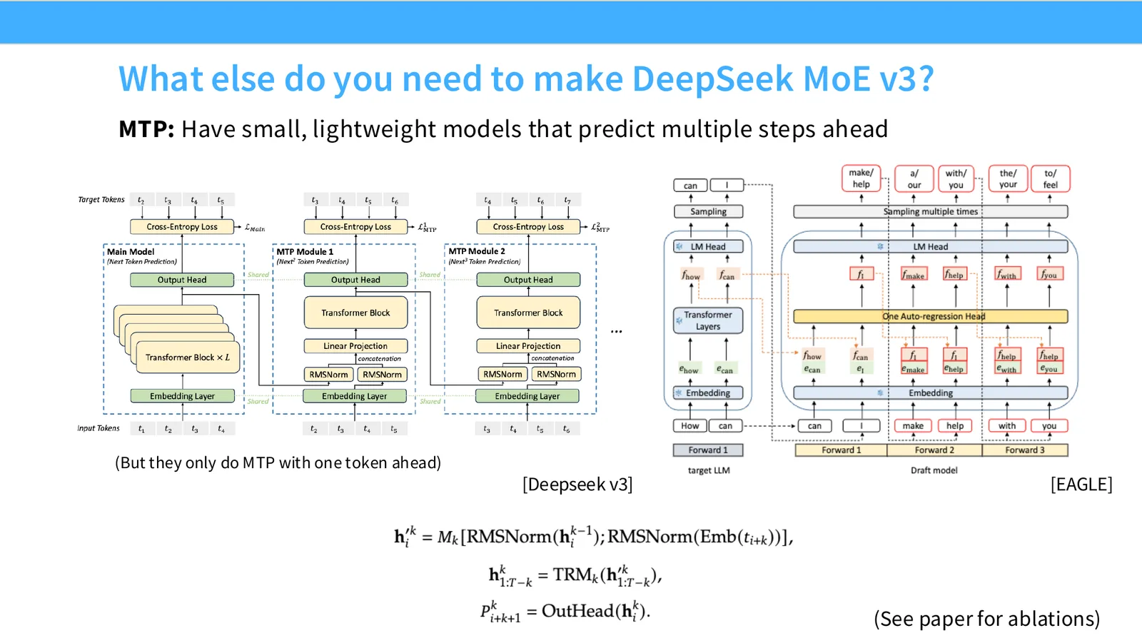
1:24:42 The only complexity that you might need to worry about is that this is going to conflict with a rope when you do sort of KV caching. So you have to be a little bit careful about how, you know, you rotate different dimensions and so on. And sort of the trick is you have non-latent dimensions that encode positions. But I'm sort of not going to go into too much more details about that. Finally, something that I thought was a very cool idea for MOE, or deep seek MOE v3, but hasn't caught on very much, is the idea of MTP or multi-token prediction. Instead of predicting one future token, you predict multiple tokens all at once. That has sort of statistical arguments for why that's a good idea. Maybe it lets you predict the future a little bit better. But also there's this nice systems argument that you kind of now have a speculative decoder built in. #

1:25:30 Percy will talk about that when he talks about inference later. #

19 MoE 总结

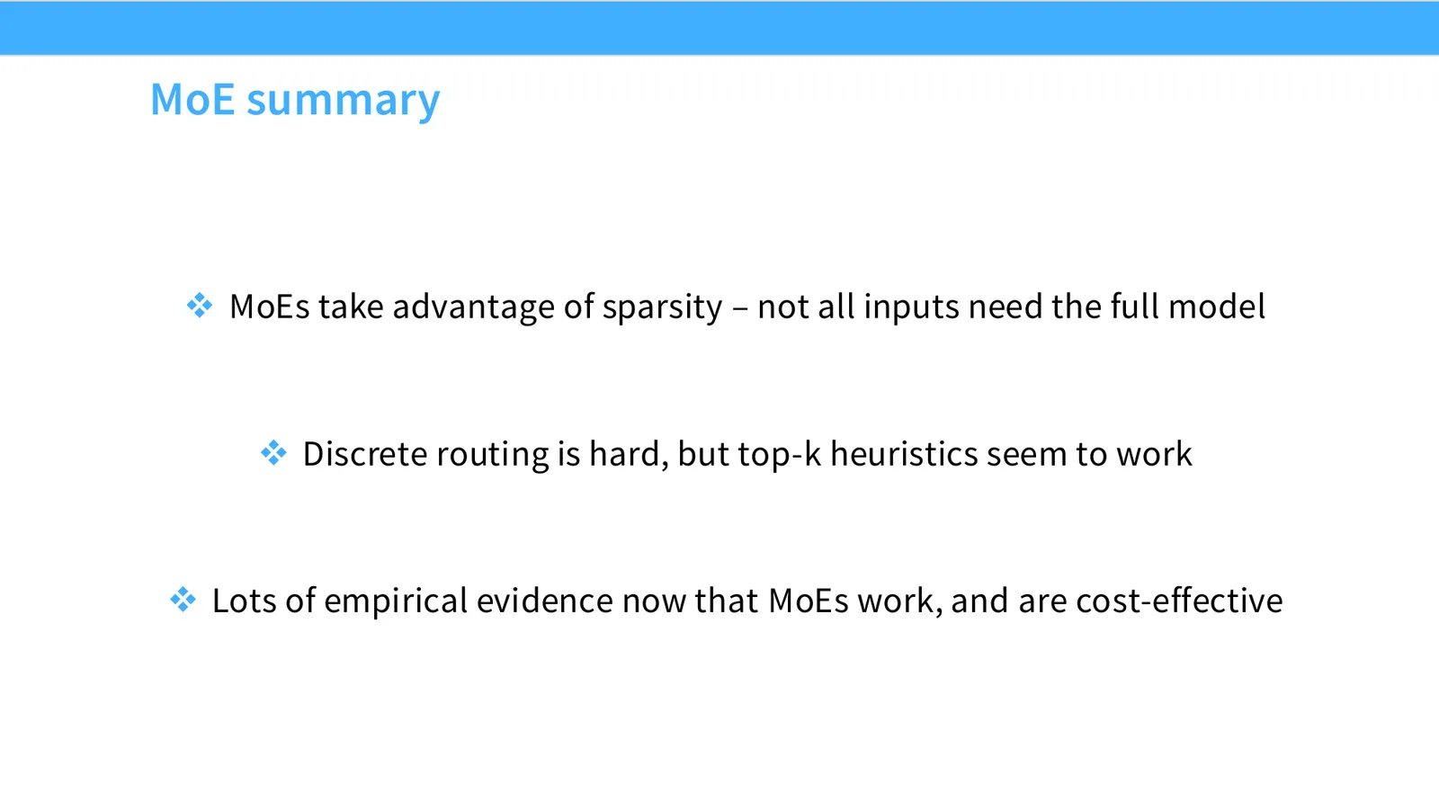
1:25:34 But it's a sort of a trick that you can use to speed up your decoding from your MOB. Okay, I think we're roughly at time. So to put everything together, right, MOEs are this kind of very clever idea to take advantage of sparsity, so that you can have more parameters than you're sort of paying for, right? So you don't pay for the compute cost of all of your parameters, but you are getting the parameter benefits. You might initially think that this kind of routing problem is very hard, but it turns out that very simple things work well even at scale. And at this point, it's kind of clear that MOEs are here to stay. So you should kind of understand how they work and what they are. Thanks. #