GPUs, TPUs

01 开场与今日组织

0:04 . Okay, we will get started. Now we're going to start the systems portion of the class. So we've been doing a bunch of neural network stuff for the last two lectures. And now we're going to start getting into GPUs, parallelization, and inference. And systems, I think, is going to be, I think, part of the stack that is most reasonable in a way. In the sense that you can like reason through all the pieces, and there will be kind of like logical steps that you can go through to get the results. So it's very different and satisfying. But when you first start interacting with GPUs, it will feel a little bit like both magic and like a very strange device that you're interacting with. #

0:48 I don't really know, as a kind of class survey, how many of you have taken like a GPU programming class of any kind? Okay, so this is pretty good. That's like a fourth, maybe a little bit less. But I think when you first interact with these things, it's actually a little bit of magic. So it's good to understand. And I think, you know, deep neural networks feel like magic, but also GPUs can too. Sometimes people will show you plots like this. Part of this lecture, I think my promise to you, is that by the end of this lecture you will understand what this plot is, or why this plot looks the way it does. And this is, you know, how much throughput you're getting on a matrix multiply, where the x axis is your dimension. #

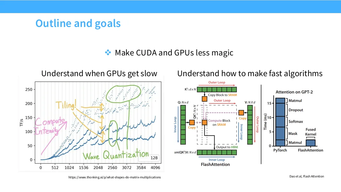
1:28 And you might think, well, you know, maybe bigger matrix multiplies are always more throughput because you have more work to do. Well, you've got all these kind of crazy patterns happening. Where like at certain sizes, your map moles are much, much slower than others. Why? You know, you'll need to understand that. You also need to understand some basics of how to sort of mentally think about a GPU in order to build fast algorithms. And even if you're not a systems person, I think probably not all of you, or even a majority of you are systems people. But if you're thinking about architectures, or just generally reasoning about these things, you kind of need to understand the hardware model of how your, you know, model is going to execute in order to make an effective model, right? Thinking back to Percy's initial lecture, right, big part of scaling is making sure you use your resources effectively. #

2:14 And without understanding your systems, you will never be efficient at using your resources. #

2:20 And, you know, I am not a systems person, surprise. And so before I start, I want to, you know, make sure to point you towards resources that I think are very good and very useful and that I used in making this lecture. Horace, he has, you know, really incredible blogs and explainers of, you know, how GPUs work. There's an enthusiast group, CUDA mode, that loves to talk about GPUs and CUDA kernels and so on. And there's a TPU and now, what? They're GPU mode now. They can use their name. Okay, fine. GPU mode. #

2:53 And the TPU book, but now it's also a GPU book by the Google folks. Actually, this is a really incredible resource. So if you're really excited or interested by any of the stuff I talk about today, I would strongly encourage you to look at that book. And they also have exercises that you can work through. And your assignment will have things that look a little bit like those exercises. So you can get a little bit of a preview of what we will send you to later. #

02 从 compute scaling 到 GPU vs CPU

3:18 Great. Okay, so this lecture is going to be in three parts. The first part is really, I would say, just like broad introductory material on GPUs. This is going to be just the hardware model, just how the programming of the GPU kind of works. Because GPU is kind of a foreign device, and I want you to understand philosophically how they're different from CPUs. And then once you do that, we're going to talk about, I think, six different tricks, important tricks to get a GPU to go fast. These are just kind of building blocks of how you can start to manipulate your code in order to make it run efficiently on a GPU. And then finally, the last part where we put all of this together is going to be, we're going to walk through flash attention. And this will be kind of our victory lap. #

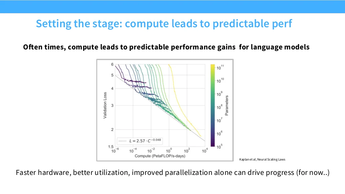
4:00 We will say, actually, at this point, we understand everything we need in order to, you know, reinvent our own flash attention and to understand all the different components. So that's going to be kind of the goal that we're going to be building towards by the end of lecture. Okay, so we haven't gone to scaling yet, but from Percy's introductory lecture or just generally following language modeling, we kind of know that if we have more compute on hand, we can get better language models, right? This is kind of the currency by which we operate. So if we have faster hardware, or if we have better utilization, or we have more chips, and then we have improved parallelization, all of these can drive progress, right? And so in some sense, the game for the last few years has been, how can we bring more compute to bear in training models? And I guess in the last year or so, how can we bring more compute to bear in the inference of these models, right? So compute is just extremely important, and systems is part of that. So if we were talking about this in the 90s, I think the things that we would be focusing on is clock speed, right? #

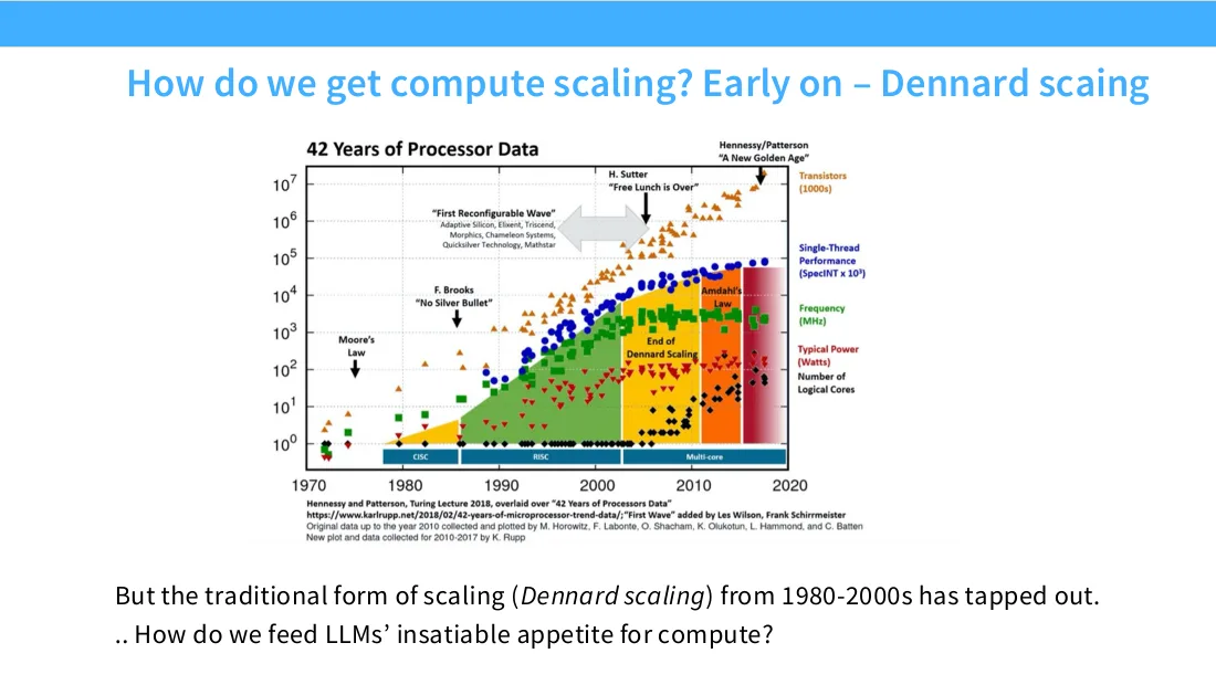
5:01 We would be saying things like, well, you know, how we make computers go fast is we have a CPU that executes instructions serially, and we make those instructions go faster and faster, right? I mean, this type of scaling, where transistors got smaller and clock speeds got faster, you know, called Dennard scaling, held quite well for a while. Really, the 2000s was about when this kind of scaling tapped out. And one sort of interesting side note, right? The number of transistors, of course, has continued to go up, but making transistors smaller does not necessarily mean that your transistors go faster, right? They don't move at a faster clock speed. There's fundamental physical reasons why, you know, you don't actually continue to get benefits of smaller and smaller transistors at a certain point. So this old approach of like making your clocks faster, making instructions execute faster is not going to work, right? So how do we, you know, get LLMs to continue to scale in this world where we can't just make things faster in sort of this frequency sense? #

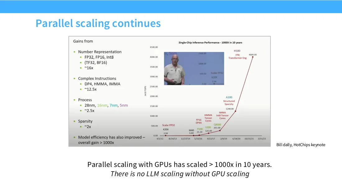
5:58 Right? And that's, you know, where the GPU shows up in sort of parallel scaling in general, right? Percy's going to talk about sort of more advanced topics next lecture, but after that's going to be parallelism, right? Parallelism and GPUs are both kind of part of the same paradigm. Instead of making things go faster serially, with your clock going faster and faster and faster, instead you're going to, you know, scale horizontally, right? Have more things executing your instructions in parallel. And so this is kind of the story of GPUs. This one slide really, I think, or one picture summarizes, you know, the state of parallel scaling, which is, you know, in the early days of, you know, K20s and M40s, you had, you know, respectable but somewhat pitiful by today's standards, flops. And all of a sudden around P100s and V100s, this curve takes off and you get super exponential scaling in the amount of floating point operations that you can do sort of year by year, right? #

6:49 This is kind of a remarkable plot in the amount of compute that we can bring to bear. And so, you know, GPU scaling has really driven almost all of the compute scaling that we've seen. And we'll talk about all of the different components that we have here. You know, I'll highlight them here just to put them into your head. You know, at the V100 era in 2017, we start getting tensor cores. That's one of the big hardware innovations. And then in the next few years, we're seeing, you know, structured sparsity and FPA and all these sort of lower number formats also driving our flops forward. And we're going to see sort of what that means in detail in a little bit. #

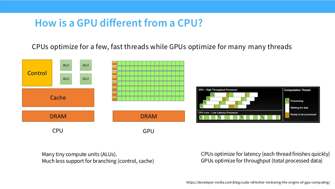
7:31 So how is a GPU different from a CPU? Those that have, you know, interacted with a GPU already know this. We'll move on to more advanced things in a minute. But for the rest of you, I think it's very important to understand the model, like the philosophy in some sense, of how they're different. So a CPU is designed for quick serial execution where you have sort of complex branching logic, complex conditionals, complex control flows. Because of this, a CPU, generally speaking, has really big control units. And it has a few ALUs that can do sort of mathematical or other operations. But this is meant to run very quickly, right? So you want to go as fast as possible and sort of have low latency. #

8:07 The time between when you get an instruction and when you complete it should be very, very short, right? That's kind of the general CPU design philosophy. In contrast, the GPU is really about throughput, right? And, you know, the plot on the right, I think, is a great pictorial illustration of when you change these philosophies, what you end up getting. So in a GPU, maybe you dispatch a task, it takes a long time for it to finish, right? It might be that you process a task and then you stop and then you go work on another task and then you go back and work on another task. But in general, right, even though your tasks don't finish quickly, you know, you're getting large aggregate throughput across all of your tasks. And what enables this is having tons and tons of lightweight cores, right? So a GPU has hundreds and hundreds of sort of compute units that are sort of packed into a chip, and all of these can execute in parallel, right? #

8:55 So this is a very different mode of programming and thinking compared to a CPU. Okay? And I want to demystify what a GPU is. I don't want you to think of it as like a, you know, set of pieces of text on NVIDIA SMI. I want you to like be able to sort of visualize what the hardware is of a GPU. #

03 GPU 解剖：SM / warp / 内存层次

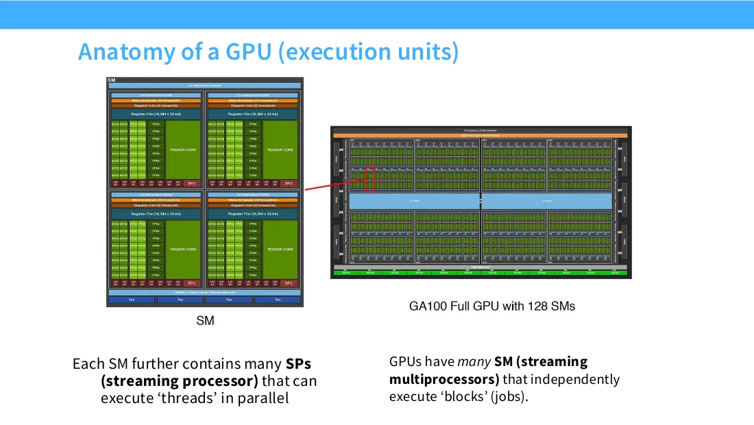
9:16 I think this picture is, I think, usually used as a pictorial illustration of what a GPU is. I think this is a great logical picture of what's happening inside of a GPU. So a GPU, the basic unit of a GPU is SM, a streaming multiprocessor. And a streaming multiprocessor is kind of like a core. It's its own independent compute unit that has, you know, subcomponents that it can use to accelerate its computation. And it has access to certain kinds of memories that it can connect to. All right? So each SM, you know, building on this idea of parallelism, it's not a single sort of compute unit. It has streaming processors inside of it that can then execute different threads in parallel. #

9:56 But SM is kind of the discrete compute unit. We'll see why later when I get to the programming model. Each SM you can think of as kind of a core almost. And GPUs have tons of SMs. Like A100 will have 128 SMs. Each of these can be independently programmed and they can independently execute different jobs. And they have access to sort of global memory outside of it. #

10:21 And the other thing that we will see, that's kind of the sort of compute story of a GPU. But we will see throughout this lecture that a really, really important part of this story is not just the compute part, but the memory part, right? Modern sort of hardware and LM optimization is really defined by the memory. And so we need to understand what the memories are and where they live. So when we talk about memory, there's different kinds. There's different levels of caches that are connected to a GPU. There are registers which are even more limited and even faster. And then you have global or high bandwidth memory. And as you can kind of see from this table, this is a benchmarking that some folks did of, I think this was the A100 latencies. #

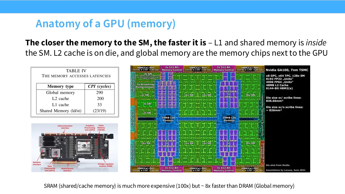
11:06 You know, the L1 and shared memory, these are very fast, right? In something like 20 to 30 cycles, you can kind of read and get data from them. If you're hitting the L2 cache, much slower. And if you're hitting global memory, you know, that's 10 times slower than the L1 cache. This is a big difference in your speed, right? And this global memory is kind of what you normally think of as a, you know, high level programmer as a GPU memory, right? When an H200 tells you I've got 144 gigs of memory, you're talking about global memory, right? You're not talking about shared or L1 cache. Now, physically, where do these things live? #

11:39 Well, global memory, you know, usually are these kind of memory chips that live outside of your sort of compute unit. Whereas L2 and L1 cache, they kind of live physically in the chip itself, right? So this is kind of the picture of a GPU chip. And you see all these SMs, these green blocks are SMs. And you see L2 right here, and the L1 is inside of each of the SMs, right? So they're physically much closer to the compute units. That's why their latency is so much better, right? And you might say, okay, then if shared memory is so nice, why don't you build a whole chip out of shared memory? It's much more expensive, hundreds of times. #

12:19 It's also much more power hungry, right, from the way that these memories are built. And so this is the reason why if you're building a practical accelerator, often you don't want to just, you know, have a giant amount of shared memory. You want to have the sort of hierarchy of memory, right, and use it effectively. I think Grok, right, which was recently acquired by NVIDIA, was a design where you just had the giant amounts of SRAM, right? And for certain workloads like inference, this is very helpful. But still, for most accelerators, you're going to have this hierarchy that you're going to really have to respect in order to make anything run fast. Yes? What is the difference between the shared memory and the L1 cache? Yeah, so the shared memory is, you know, and the L1 cache, I guess, kind of operate differently. #

13:04 The cache is really just a cache thing that is storing recently accessed data elements. Shared memory is a programmable element that you'll actually interact with, that you can, like, put things in and out of. #

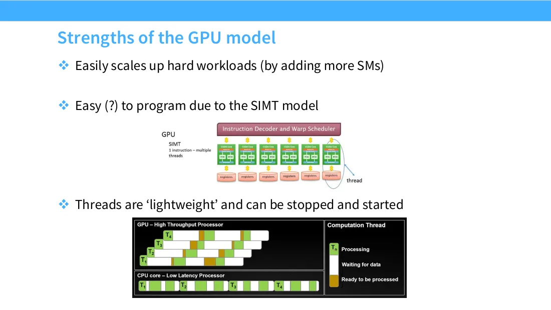
13:18 Okay, cool. Right, so that's the memory story, and keep that in mind, because it's going to keep coming back, the memory hierarchy. That's a really important object. Now, okay, we have the hardware mental model in place, and now we're going to start talking about the software and programming model of the GPU. So there's three different important players that live in the execution model of the GPU. So there's a thread, and if you're familiar with multi parallel programming of any kind, you know what a thread is, right? A thread is a sort of lightweight thing that's running in parallel and doing some work, right? In a GPU, an important thing about the threads is they follow the SIMPT model, which means that all of the threads that you have are executing the same exact instructions, right? They're going to have different inputs, which means that the threads can actually do separate useful work, but the instructions they execute have to all be the same, right? #

14:11 And this has important implications for both the efficiency of your code, as well as the programming model, right? If the threads can do all sorts of different stuff, it becomes very hard to program, right? GPUs are this trade-off between programmability and efficiency. Now, a block is a group of threads, and the reason why a block is a relevant object is that a block is guaranteed to run on a single SM. And remember, an SM has a shared memory, and so you can think of a thread as doing work in parallel. Blocks have access to a shared pool of memory. That will become very important later when we talk about this idea called tiling, where these blocks are going to be reusing the same pieces of memory. Finally, a warp is essentially kind of the scheduling unit of what is happening inside the GPU. Threads are going to execute in groups of 32 consecutively numbered threads. #

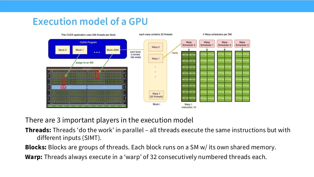
15:03 That is a warp, right? This decreases the overhead of a scheduler deciding which threads to run. But essentially, these are kind of the important three terminology items for a GPU. I might say something like, oh, you know, we're going to have different warps executing. That's what I mean here. That's a basic unit of 32 threads that execute together. Yes? You mentioned that all threads execute the same instructions. So is it all threads in a block or all threads in a warp? #

15:27 All threads in a warp are going to be executing. #

15:32 Cool. Yeah? So the scheduler decides which warp the next instruction goes to? That's right. Or sorry, the scheduler decides which warp is going to be executing next. #

15:44 And on one assignment and so on. Cool. Okay. And so in the memory model of a GPU, device code can read from registers. Registers are some of the fastest and most local items. This might be storing things like memory addresses of where you might need to, your arrays start and end. That's a place where you might store things in registers. Then you've got local memory. This is local to within your single SM. #

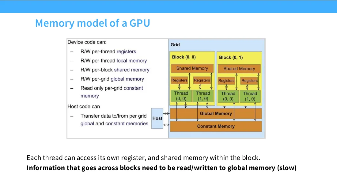
16:11 You've got shared memory that can be accessed sort of within your block. So if you have something you want to transfer across threads, or you want to have information that is going to be reused across threads, those are going to live in shared memory. You can of course then read out, or sorry, read from global memory, right? The, the DRAM that's far away. As long as you're willing to pay sort of the latency hit of waiting for data to come to you from global memory. And there's also sort of constant memory, which I don't think I've seen very much used in, in various programming things, that you can use as well. Now, you can even sort of transfer to and back from host memory, right? When I say host memory, that means sort of CPU memory that lives on the machine. You can do this if you need to offload beyond the size of your GPU. #

16:55 This is kind of the set of things that you can do in your memory, right? And, and really the key thing, the most important part of this, this sort of memory model is that as soon as you go outside of your shared memory, things are going to be slow. #

04 插曲：TPU 与 GPU 的异同

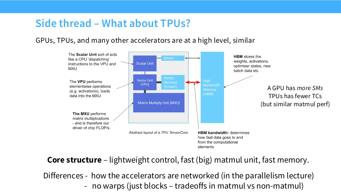
17:08 So grouping the blocks to sort of decrease the amount of global memory reads is going to be the name of the game throughout this lecture. Okay, now I'm going to talk for two slides, two slides about TPUs. The majority of this lecture is about GPUs. Mainly because I think, you know, if you all go out and you, you know, write your code and you build your models, it's probably going to be on GPUs for most of you. But I think it is very important that we talk about TPUs, both because I think TPUs are cool and becoming more popular, but also because TPUs are kind of like the alternative evolution of GPUs. And you can kind of see what's the same, what's not. It's very interesting to see how TPUs work as well, right? So, actually what's very interesting is that TPUs are very similar to GPUs at a high level. This is kind of convergent evolution. #

17:59 If you want to build a energy efficient accelerator that does machine learning, you kind of end up at the same place. So the core mental difference between a TPU and a GPU that you should kind of keep in mind is that TPUs are in some sense simpler. They're more optimized for the machine learning workload. They have light or weight control units. And they have much bigger matrix multiply units. And so, you know, they have the same basic structure that I'll talk about for, for, sorry, for GPUs, where they will have a specialized circuit to multiply matrices. They will have components that can do parallel vector operations. And they will have, you know, some control system. They have a very similar looking memory structure where they have slow memory, which is called high bandwidth memory. #

18:47 And then they have an even faster local memory called SMEM or shared memory, right? So this looks very, very similar to the architecture of a GPU. Really, the difference is in how these things are sized and the flexibility of these operations. And I would say, oh, and the main difference that I won't get into today is the networking for these accelerators. So if you're thinking about what is the big difference between a TPU and a GPU, actually the biggest differences come in networking, not in the individual chips. Because really the chips, you know, they live to just multiply matrices. #

19:20 And this is from the Jack's book, you know, which is a really lovely resource. But they have these two tables. They have a section on GPUs where they describe how to essentially map GPU ideas to TPU ideas. And whatever I say today about what's on the left here, you know, you can map directly to the TPU. But the important thing, you know, at this point in the lecture to notice, is that for every sort of concept in the GPU, there's a corresponding concept in the TPU. And this, you know, mapping is actually pretty precise. Like a tensor core in a GPU, which is the matrix multiply unit, corresponds almost exactly to an MXU, which is a matrix multiply unit in the tensor core. And if we're getting into really nitty-gritty details, they actually use the same underlying, you know, like circuitry, right? They're both what's called a systolic array, which kind of streams data in and out to do a matrix multiply. #

20:07 So the architecture is very similar. Now, how are they, oh, sorry, yes? Do you know like what a typical systolic array size is on the GPU versus TPU? Ooh, I do not know that off on my head. I'm sorry, I'll have to look that up. Yes, just a little bit. Okay. So the main difference between these two is the number of different units that we have. So if we look at, oh, actually, I'll mention one very, very confusing thing before I move on, sorry. #

20:35 TPUs call their streaming multiprocessors tensor cores. GPUs call their matrix multiply units tensor cores. They are named exactly the same thing, so you will have to disambiguate them based on context. If someone says tensor core for TPU, that means a processor. If someone says tensor core for GPU, they mean a matrix multiply unit. So if you look at a GPU, a typical GPU, like a H100, might have something like 132 streaming multiprocessors. It's a lot of processors. A TPU will only have two units, right? There's only two separate units running in parallel. #

21:08 Now, the GPU, if we just look at the matrix multiply units, will have 528 matrix multiply units, whereas a TPU will have just eight, right? And these are roughly scaled to be comparable looking objects. Why is it that it's this way? Well, the TPU is relying on much bigger, smaller numbers of matrix multiply units, whereas the GPU is relying on smaller but much more numerous matrix multiply units. And you can kind of imagine that if you have a small number of many matrix multiply units, it's going to give you more flexibility. You can program them to do this and that, whereas a TPU, you're locked in to big, big matrix multiplies, right? And so there was a funny situation in a recent paper that I wrote where, you know, we did a batch size sweep and it goes all the way down to 64 and it stops at 64. Why is that? Because the tensor core refuses to accept anything smaller than a 64 dimensional input there, right? #

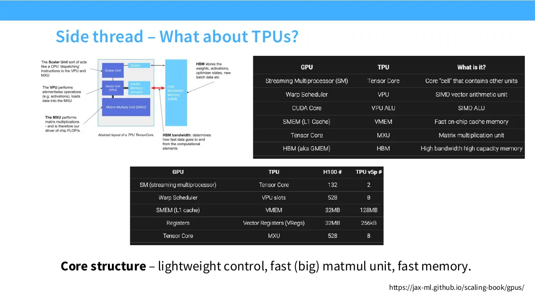
22:00 It has to be big matrix multiplies. So this is the main difference, but as you can see, GPUs and TPUs share a lot of similarities. They rely on a memory hierarchy between fast memory and slow memory, and they have a matrix multiply unit. And because of that, the core concepts that I'm teaching you today is going to transfer over between GPU and TPU, right? The basic ideas are always going to be the same for that reason. And this is really convergent evolution. There are only so many ways to sort of cost effectively allocate memory, and there's only so many ways to multiply matrix very fast, right? There's some design decisions that are different, but otherwise you end up at the same place. Okay, cool. #

22:37 So that's TPUs. And right, good. And GPUs, I think, have been enormously successful because it allows for, you know, easy scalability for things like matrix multiplies. If you want more throughput, you just keep adding SMs, right? As long as your memory bandwidth can handle those SMs, you get more and more throughput. The programming is, you know, something we don't think about, but it's deceptively easy, right? If you were to try to write, you know, lower level machine code looking stuff like PTX, it's actually doable because it's all SIMPy, right? It's not like you're programming every single thread. You know, you're saying, okay, here are my instructions. #

23:14 Here are my inputs. Now run them on all of my inputs, right? It's something that maybe you all are already familiar with, with things like applying or using functional programming. #

23:25 Finally, I haven't talked much about threads, but whenever you're doing GPU programming, these threads are always very lightweight. They can be stopped, started at any time. The scheduler can decide that, okay, I have another warp that's, you know, better to run, so I'm going to stop you and start this one. And it's very sort of quick to sort of swap in these jobs. That allows for much higher throughput if certain jobs are stalled or have some property that's lowering throughput. #

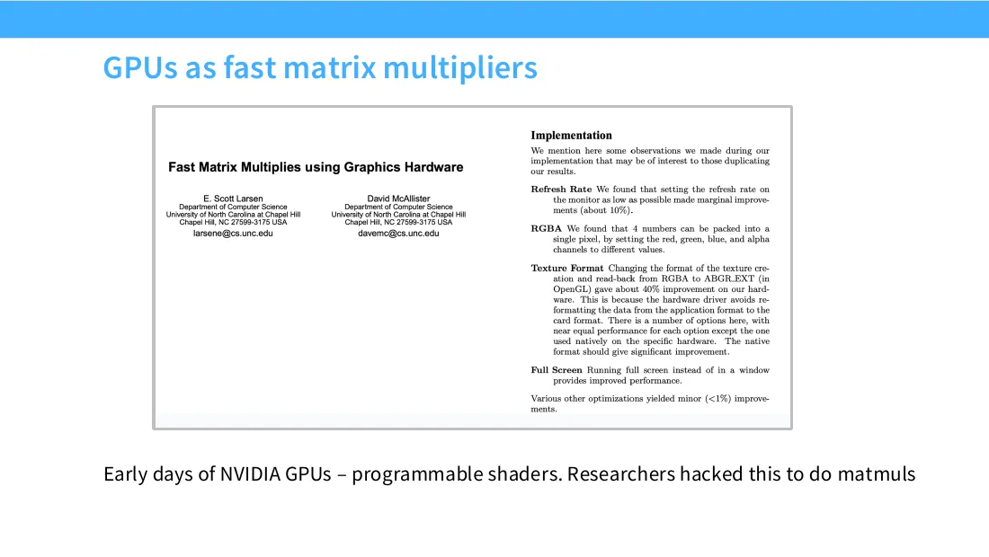
23:51 Okay, so that's the benefit of GPUs, you know, as a hardware model. It's been enormously successful. And I think even in the early days, before tensor cores sort of were implemented, you know, people realized that, you know, commodity graphics hardware, this massive parallelism, would be very effective for, you know, scientific computing. So, you know, this is one of the original papers on using graphics hardware for fast matrix multiplies. And this is really, really cool sort of hacker work. You know, people figured out, well, we have these shaders that are implemented, but we can program specific shaders that will actually work. So, you know, actually give us sort of matrix multiplies and different rendering settings actually give us faster matrix multiplies. And that's just sort of really cool computer science things you can do. But nowadays, you do not have to do this. #

24:36 You do not have to manually program your GPUs to do matrix multiplies. #

05 GPU 模型的优势与 tensor cores

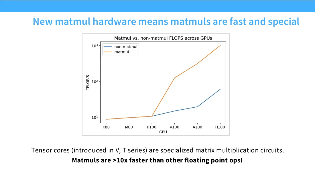
24:40 Because as of the V100, NVIDIA decided, you know, here is a piece of hardware that will do your matrix multiplies for you. And once that hardware sort of existed, MATMULS became the sort of one privileged operation in machine learning, right? So at this point, there's a gigantic gap in sort of the throughput that you're going to get between sort of parallelizable but non-matrix multiply operations versus amount of operations you can do in a matrix multiply, right? So this is one of the reasons why sort of any near future machine learning architecture that we see that scales with compute is going to have a matrix multiply in it, right? Because this is the one way that you can really effectively get a lot of compute throughput. #

06 Memory wall 与 Part 1 小结

25:23 More than 10 times faster than any other floating point operation that you can do in a GPU. #

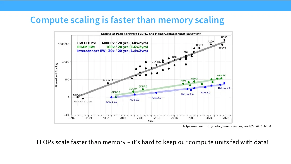
25:31 Okay. And then the last sort of hardware thing that I'll end with, I think this is the last slide of this section, is that different components of the GPU are scaling at different rates over time. We know that the GPUs are getting faster and faster, this is just like a thing, right? As well as CPU, you know, overall compute throughput is getting faster and faster. So that's the gray line, right? That's pretty fast. We're getting faster and faster improvements in the total floating point operations. Green is our memory bandwidth. This is how fast we can transfer data. #

26:03 That's growing comparatively slowly. Blue is parallelism. This is how fast we can connect different GPU devices. That's also going very slowly. And what does this mean? This means that if you're out here kind of in the early days of GPU programming, probably you weren't thinking much about memory. Because your compute wasn't that much faster than your memory transfer. But now as we go more and more to the right of this plot, we're going to see a bigger and bigger gap between compute and memory. And that's why a lot of the optimization I'm talking about today are memory optimizations, right? #

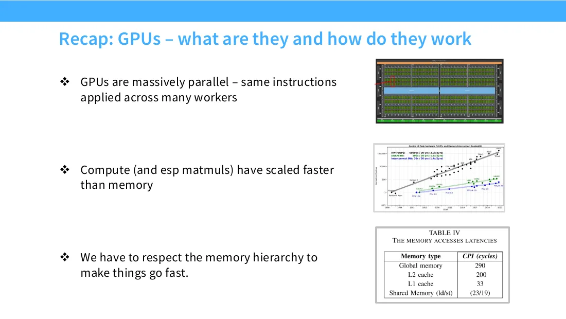
26:33 As we go further to the right, we're going to see memory and communication bottlenecks more and more. And so it's going to take more and more work to fully utilize the hardware that we have. Okay. So that was our sort of very basic overview of GPUs. I can't possibly, you know, give you a 20 minute lecture that fully helps you understand what the GPU hardware is. But hopefully you have a flavor, right? The mental model should be GPUs are massively, massively parallel. They execute instructions all at the same time. Compute scales really fast, really, really fast, and even faster than memory, which means memory is really important. #

27:09 And because memory is important, everything we do has to respect the memory hierarchy, right? As much stuff that we do goes into shared memory and not global memory, right? So this is kind of hopefully your understanding of GPUs. And if you have this understanding, at least you'll understand all the basics necessary to internalize the next part of this lecture. Okay. I can pause for a moment here in case people have hardware questions or anything else before I move on to the next part. Yes? So, before V100s there was no matrix multiply unit? Yeah, there was no tensor core that like specialized to a matmul. #

27:46 Yeah, the tensor core is a V100 edition. Before that you would be programming manually. Of course, you have so many SMs and so many like ALUs that you can still do quite good throughput. But, you know, a specialized circuit for matrix multiplied really, you know, changes the game for that. Oh, yeah, back there. What is the difference between the shared memory and the L1 cache? The cache just operates on its own. Like you don't get to control the L1 cache. #

28:11 Is L2 slower than L1 just because of the physical distance or does it also differ some other way? Yeah, I mean physical distance is a big part of it. I mean they are, if I believe, if I remember right, they're both SRAM. Like that's one of the reasons why global memory is much slower. But the physical distance and the interconnects that are used are the reasons why it's slower. Yeah, this is not inherent by the way. One additional side thing is that the equivalent L2 cache in TPUs is much faster. Because they make different design trade offs on silicon to enable that. That's one of their selling points. #

28:44 Yes? If the compute memory gap keeps growing, do you think that affects the way future chips will be laid out? Yeah, or maybe the future chip kind of budget splits. One of the things that I really didn't want to talk about, but now you forced me to, is kind of the inference landscape for hardware is actually even more crazy. So one of the things that people started doing, I think last year, was something called pre-fill decode disaggregation. Where the pre-fill part, which is very heavy matrix multiplies, is one chip. And then the decode part for your inference, which is more memory bandwidth limited, is another chip. Right? And some of the models, I think this was Stepfun3, which is a Chinese open source model, even has a thing where they try to disaggregate different layers. #

29:31 So an attention will go to one chip optimized for one thing, or one accelerator. And then MLPs will go to a different accelerator. Right? And so you're starting to see, like, if this gap grows, any sort of clever tricks to utilize your very precious, fast memory becomes very valuable. And you start to see this very heavily in inference, which is even more memory bound than training. Yeah. Cool. Oh, yeah. How many warps are in a block? #

29:57 How many warps are in a block? Do I know that? I don't think I know that. #

07 Part 2 开场：roofline、六大技巧与 control divergence

30:03 I think it's also hardware dependent. Okay, good. #

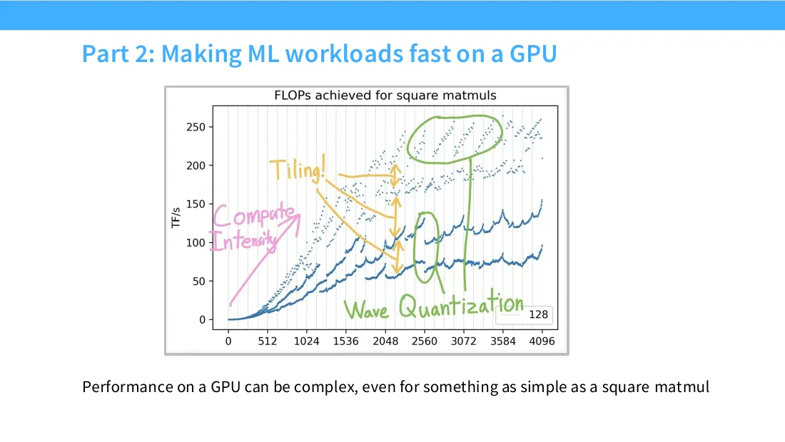
30:09 Okay, so the second part of this lecture is now you all have a general sense of what a GPU is and how it works. Now we are going to talk about all of the basic tricks to make workloads fast on a GPU. These are kind of basic components that you can kind of put together to make things fast. And to keep us kind of motivated, one of my goals by the end of this section is to explain this plot to you. Right? So this plot, as I said before, has a very simple picture. It's the size of the matrix, a square matrix that I'm multiplying. I'm multiplying two square matrices. And this y-axis is how many items I'm processing per second. #

30:45 So this is the throughput, right? And as I'm going to the right, in general, throughput is going up because I have bigger matrices. I have more work to do. And so, you know, if I have a lot more work, I can keep my hardware more utilized, right? But there's all sorts of strange patterns here. And we kind of want to understand why are there strange patterns here? And how can we be at the very top of that curve rather than the bottom? So that's what I'm going to be talking about in the second part. Okay. #

31:10 And, you know, Percy already mentioned this. This is the roofline model. But the plot I showed before looks a little bit like this classic roofline model, right? This looks like there's a diagonal part and then a flat part, right? And this is what we expect, right? The roofline model says up until a certain point, we will be memory limited, right? We're memory limited, so no matter how much, you know, compute you give me, my sort of throughput is not going to go up. At some point, you have enough work per unit sort of memory movement that I can keep sort of my compute units completely saturated. And past that point, having bigger and bigger sort of units of work does not help me anymore, right? #

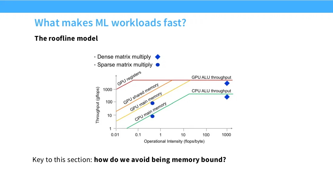
31:50 No matter how much sort of extra work you give me, that doesn't help because, you know, I fully saturated by matrix multiply units. So this is what we expect out of the classic roofline model where, you know, as we sort of have faster memory, we can kind of push this upwards. But there's a memory bound region, which is diagonal, and then a compute bound region, which is flat, right? This is kind of what we expect. Now, if you want to make sure that your code runs efficiently on a GPU, really what you need to do is you need to be on this flat part, right? As soon as we have this flat part, there's nothing else to do. We're at maximum throughput, right? So we want to prevent ourselves from being in this diagonal part, which means we want to increase the operational intensity. The amount of computation we do per memory read needs to be high enough. #

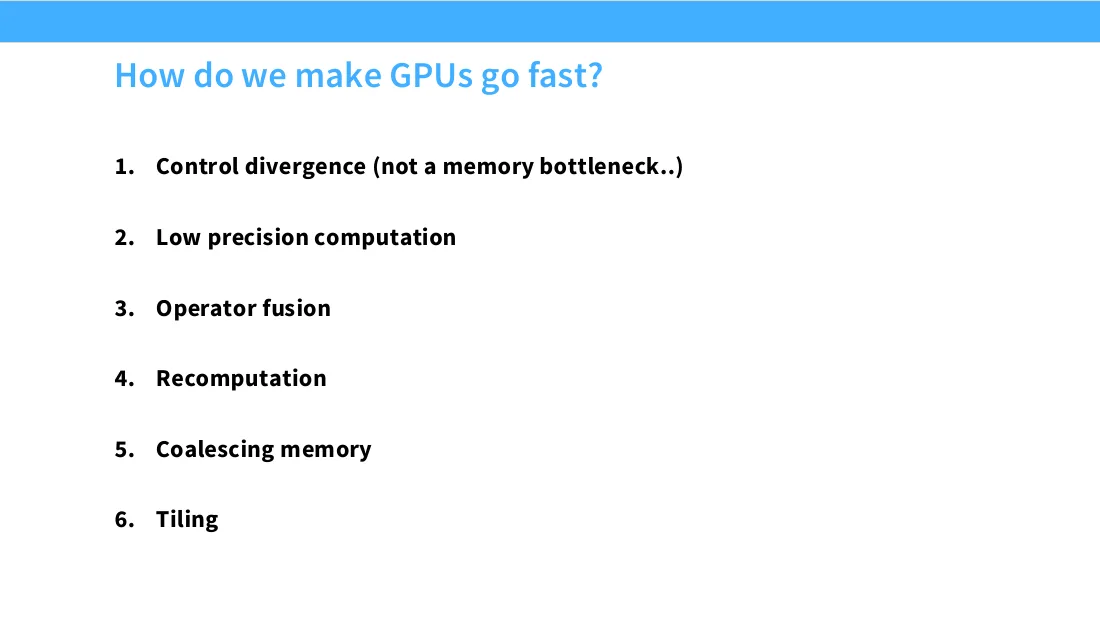
32:34 So that's what we need to do. And there's six different tricks that we will talk about. Actually, some of these are not sort of memory tricks, the first one only. There are six different tricks that are maybe necessary to understand to make GPUs go fast. The first one's a little bit different in flavor, but then the rest of them will have this flavor of trying to minimize memory movement as much as possible. #

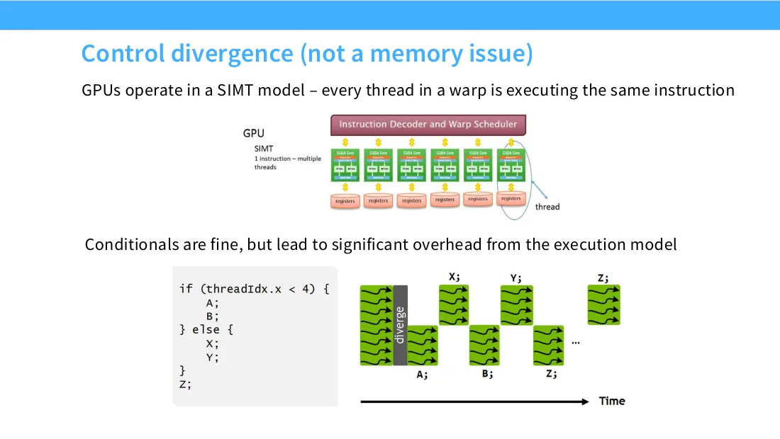
32:57 The first one is kind of a GPU-specific thing, and it relates to one of the things I said before, the SIMPTI model. So in a GPU, every thread is executing the same thing. Now, what happens if you write an if statement on a piece of code that executes on a GPU, right? On a CPU, it's quite clear what happens. On a CPU, you will either pick one branch or the other. You will execute that branch, and you will move on with your life, right? In a GPU, you will do something actually quite different and slightly counterintuitive. Every thread has to execute the same instruction. So actually, every thread will kind of execute both the if and the else. #

33:35 But if you're not part of the if branch, you will just mask out that computation. You'll just sit idle, right? And so whenever you have a conditional, your mental model for the execution kind of looks like this. You know, part of your threads will diverge based on this if statement. Some of them will go to the bottom branch. Some of them will go to the top branch. And the bottom branch ones will execute first. Top branch ones will wait. And then the top branch ones will execute, and the bottom branch ones will wait. #

33:58 Right? So in order to execute an if statement, you're actually sort of walking through both of these. And then some of the threads are just waiting, doing nothing, if they're on the wrong side of the branch. And this is called control divergence. And this is nice in some ways because it simplifies programming. It's not nice in that you now have these big compute gaps where your GPU is doing nothing. Right? This is one of the reasons why you really do not want to write if statements. You know, if you look at GPU code, like if you have a ReLU, you'll often find you're like multiplying with zeros or you're multiplying with masks instead of doing like an if statement where you're updating half. #

34:34 Right? Because the multiplication is going to all kind of go up once. And an if statement might actually have to wait two clock cycles or something like this, two operations. Okay. So that's the first thing. But, you know, that's a sort of separate story from all this memory stuff, which is kind #

08 技巧 1：低精度（FP16 / FP8 / MXFP8 / MXFP4）

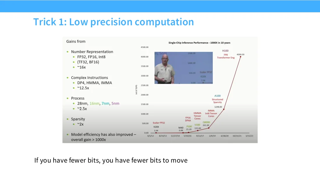
34:50 of the main narrative or the main story of this. The first one, which you don't really have to do too much for, but I think is one of the most important ones. And hardware wise, I think where Nvidia is investing the most effort is low precision computation. And if you look at this plot, I've brought, you know, Bill Daly back to the slide. This super exponential growth, where does this really come from? Actually, a pretty non-trivial part of this, you know, is number representations. You start at FP32, you go to BF16, and then you go to int8. You just keep decreasing the precision of your numbers. And of course, if you have half the bits, you have half the bits to move. #

35:30 And so you've halved your memory movement, right? And so you've solved the memory bottleneck for at least a little bit. #

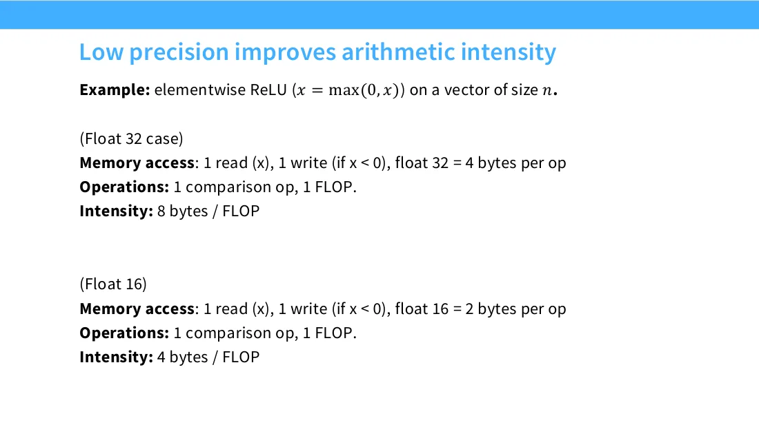
35:37 You know, this is a dumb example, but, you know, I'm just going to really drill it in there. You know, let's say I have a value on a vector of size n. If I'm on float 32, I need to do one read, right, to read my number. I need to do one write after I've computed my value. That's going to be four bytes per operation, total of eight bytes for my memory access. I only have one flop worth of operation, so that's eight bytes for a flop. You know, if I halve the precision, of course, I've halved the number of bytes per op. I've, you know, halved the number of bytes that I need to move per flop. Sorry, this is the inverse of arithmetic intensity. #

36:13 Arithmetic intensity should be reverse of this, right? #

36:19 Now, that's a very simple example, but actually how low precision works in a modern GPU is actually very complicated and actually either very cool or very crazy, depending on how you sort of think about, you know, how cool things are. So when you do a matrix multiply, let's say you have a tensor core that's operating in lower precision. How does that actually work in practice? Well, you're actually not going to keep everything in low precision. You're going to downcast before you take your product. And when you sum up your partial summons in your matrix multiply, you're going to do this in full precision. And then you might emit your outputs or your results in FP32. And part of, I think, the reason why low precision is actually kind of a black art is not because you can just like decrease precision. Anyone can do that. #

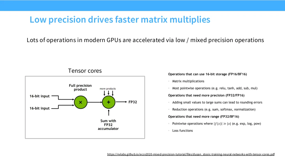
37:05 You have to figure out which of your operations has to be in which number format, right? So, you know, matrix multiplies, maybe both your weights and activations can be low precision. If I'm doing a soft max, maybe I need to do that in FP32. Or if I'm doing an exponential, maybe that also needs to be FP32 or maybe I can get away with BF16, right? So, you know, I think it took several years really to get low precision training to be the state that it is today. And a lot of that work was, you know, slow, incremental, empirical work figuring out which of these operations we can sort of downcast, how we can downcast them, and how we can preserve stability of training while making as much of our training and inference low precision as possible. #

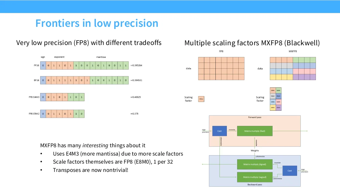
37:51 People have been pushing this further and further. I think, you know, once you think about how hard it is to pay for fast memory, you realize, if only I can cut my precision by another factor of two, right? Like people really, really want to do that. And so, you know, FP8, you know, was kind of the next frontier, I would say, of low precision. Once you get to FP8, there's no longer a standard canonical format that everyone uses. Like if you're using FP, or sorry, 16 bits, you're probably using BF16, right, for a lot of what you're doing. But with FP8, there's going to be E4M3, which stands for four bits of exponent and three of mantissa. Or there's going to be E5M2, which is more exponent, fewer mantissa, right? Because these are used in different places. #

38:36 There's no one size fits all once you start to get to so few bits. But I think the thing that's really interesting is the more advanced low precision number formats that are coming out with the new hardware. So I'll talk briefly about MXFP8, because it's both cool and what it does to training is strange, to say the least. So in FP8, the traditional version of training, what you have is that all of your, let's say, activations are in eight bits, right? So this is up here. And then you're going to have a scaling factor in 32, FP32, that's going to allow you to scale this up and down. Why do you have a scaling factor? The scaling factor is necessary because you only have four bits of exponent, let's say, right? That's so few bits of exponent, you're going to quickly over or under flow. #

39:21 So you need the scaling factor to kind of keep you in the right range so you can keep some information, right? Well, people realize this is not optimal, because a single matrix might have very different magnitudes, right? One part of my sequence might have much bigger sort of activations than another. So instead of having a single scaling factor, why don't we have many scaling factors, right? So MXFPA and sort of these multi-scaling factor formats that are sort of much more advanced now have many scaling factors. Each of these scaling factors corresponds to the relevant colored sub matrix, right? So the first four elements in this matrix corresponds to this first scaling factor, and so on and so forth. Now I have more scaling factors. These scaling factors are actually going to be in lower precision. #

40:10 These are going to be 8 bits as well. They're going to be E8M0, so they only have exponent bits. So they're all powers of two, you know, in 8 bits. So you have to make these tradeoffs. #

40:24 Now, what was I going to say? Okay, so MXFPA is going to use more mantissa in the elements. Scale factors are themselves FPA. And you're going to have one scale factor every 32 elements in your matrix. Okay, I'm going to pause here. Don't read the third thing. Now, think for a moment, what is the problem with this design? Like, what is the big issue if you do something as clever as this? #

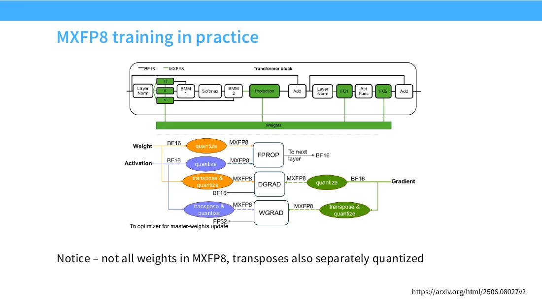
40:46 So the big issue here is, let's say I want to transpose this matrix. The transpose of this matrix does not have the same pattern, so to speak, scaling pattern, as this matrix, right? And so now, it used to be that a transpose of matrix was simple. I just transpose this matrix. I don't have to re-quantize. I don't have to do anything. Now, transposing this matrix is very complicated, because I now have to potentially re-quantize this whole matrix to fit this one out of 32 pattern that I have. And so what happens internally when you actually use MxFPA, and I found this to be crazy, but also kind of cool, is that when you're training your model with this thing, it actually creates two copies of every quantized matrix, one for your original matrix, one for the transpose. So if you ever want to transpose, you have the transpose version waiting for you, right? #

41:35 And that's kind of how you get around this, which I think is a crazy and cool thing. The point here is maybe not to emphasize the GPU trivia, but the point here is that once you start getting to these FPA, FP4 formats, things start getting pretty exotic. Because the amount of exponent and sort of mantissa loss that you have are pretty extreme. So you have to be very clever about how you do this. And as I said, if you were to go and really train a model FPA, which I think a lot of frontier labs are doing for the compute benefits, you have to be very careful, right? This plot does show kind of what I was saying. So every time you quantize, you're going to quantize one way, and you're going to transpose and quantize, so you're going to have both copies. And then the other part, which I told you about a few slides ago, is you're only going to quantize certain layers that you think are safe to do so, right? And this is another trial and error thing that you have to figure out, right? #

42:27 But once you have all this together, you have the big benefits of training in FPA, which is that when you're doing those matrix multiplies, you're probably going to get 20 to 30% savings, maybe more depending on the size of your matrix. Unfortunately, it's not going to be a 2x speedup, because you have to do all these quantization operations, right? There's a big overhead doing this, so it's not free. Yes? I remember from the reading that the first layer and the last layer are very hard to quantize. Do you have any intuition about that? That's right. That's right. #

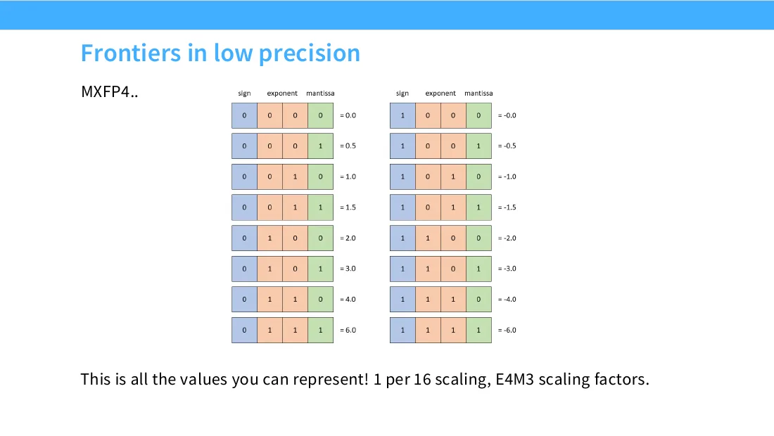
42:58 I don't know if I have intuitions for the first layer. The last layer, I think, being hard to quantize is because it is kind of a first order factor. It drives a ton of the loss. And so I think you end up getting both instability and big loss increases if you attempt to quantize the very last layer. Okay. I put this up here almost because I think it's so ridiculous. You know, the next frontier, this is already implemented as MXFP4. The entirety of MXFP4 can be shown to you in this slide. It's negative 6 to 6. #

43:28 You know, you have all the possible values. But now that you understand MXFP8, you can also understand how this thing works. You know, you're going to have a structured block where each block is going to be one of these four bits. You're going to have, every 16 of these numbers, you're going to have one scaling factor. And that scaling factor will itself be FP8. This is E4M3 scaling for those scaling factors. These are, there has been a paper that has trained with FP4. I don't think I've heard of anyone successfully training in the wild. You know, real big serious models with FP4. #

44:02 But I think this is coming, right? Like the next generation of models will probably be FP4. Okay. So that was low precision. I think it's really cool that you can really push the limits so far that, you know, you're ending up with just plus 6 to minus 6. And yet you can do interesting things with matrices in that precision. Now, oh yeah, there's a question. #

44:23 So, is this only for, like, matrices that you can apply this? Like, not just symbols that are on the screen? Yeah, so you can quantize anything. You can quantize the activations after a ReLU, for example. But there just isn't as much of a need to. So, like a matmul, if you quantize that, you can get really big throughput improvements, right? And that's why, if you look at the MXFPA training one, you know, these are all matmuls that are getting FP8 quantized. The overhead is probably not worth it for mostly of them. This is to do with, like, the hardware. #

44:57 Like, it's not like the matmul hardware part that only does this. Well, it's not exclusive to that. Yeah, like you can always do lower precision stuff, and then it will decrease your memory movement. This is true. But for the others, it doesn't quite make sense. This isn't any, like, hardware limitation. It's not a limitation, but there is hardware support for all of this, right? So it is baked in, a bunch of this is baked into the hardware to accelerate it. Yeah? #

45:21 You've positioned this as an improvement for memory bandwidth, or, well, requiring less memory bandwidth, but is there a benefit to compute as well? Yes, yes, for sure. For compute, you get basically linear improvements for just multiplying the quantized numbers. But the fact that you have to quantize and de-quantize means that the benefits are more diluted. Yeah? Do you have to train on the scaling factor? The scaling factor is an implementation dependent choice. Like, depending on the library, for example, you might get different ways of quantizing and de-quantizing. #

45:55 Training is a strong word, but you might have quantization factors that, like, scan through and pick the max min, or you might have scaling factors that look at historical running statistics and then use those. I wouldn't really call them training, per se. At inference, you might fit them more. So there are no ingredients? At inference time, you might. At training time, you would not. Yeah? Has anything been done with structured sparsity? Like, I guess,. #

46:18 Yeah, there's a lot that's been done with structured sparsity. And MOE is, I think, one successful example of a structured sparse operation that people use. What about like? #

46:30 Yeah, right. So, I mean, a lot has been done. Chris Ray here has done a lot with, you know, lots of different kinds of structured matrices. I think the benefits of that, like, you know, in terms of the compute benefits versus the representation losses, I think has kind of washed out. I don't think it's a bad idea, but empirically it hasn't, I think, necessarily panned out. Oh, yeah. A lot of like, these like squeeze that we've been talking about quantizing models in a decade. What is current SEMO approach? Is it like training in full precision or half precision and then like, distill into like quantized model that you can write on your computer, things like that? #

47:06 Like what is like SEMO approach? Yeah, I mean, there's a combination of like, you probably want to train a bigger model and then quantize down. There's various kinds of like quantization scaling laws and papers that people have written like, precisely characterizing the trade-offs here. I think the state of the art involves combining both like quantization aware training to some extent, like model scaling with post training quantization of various kinds. Like, yeah. There's a lot that I think is not fully well understood. Even industry teams that I've talked to are sort of talking about still doing like science of quantization. #

09 技巧 2：算子融合

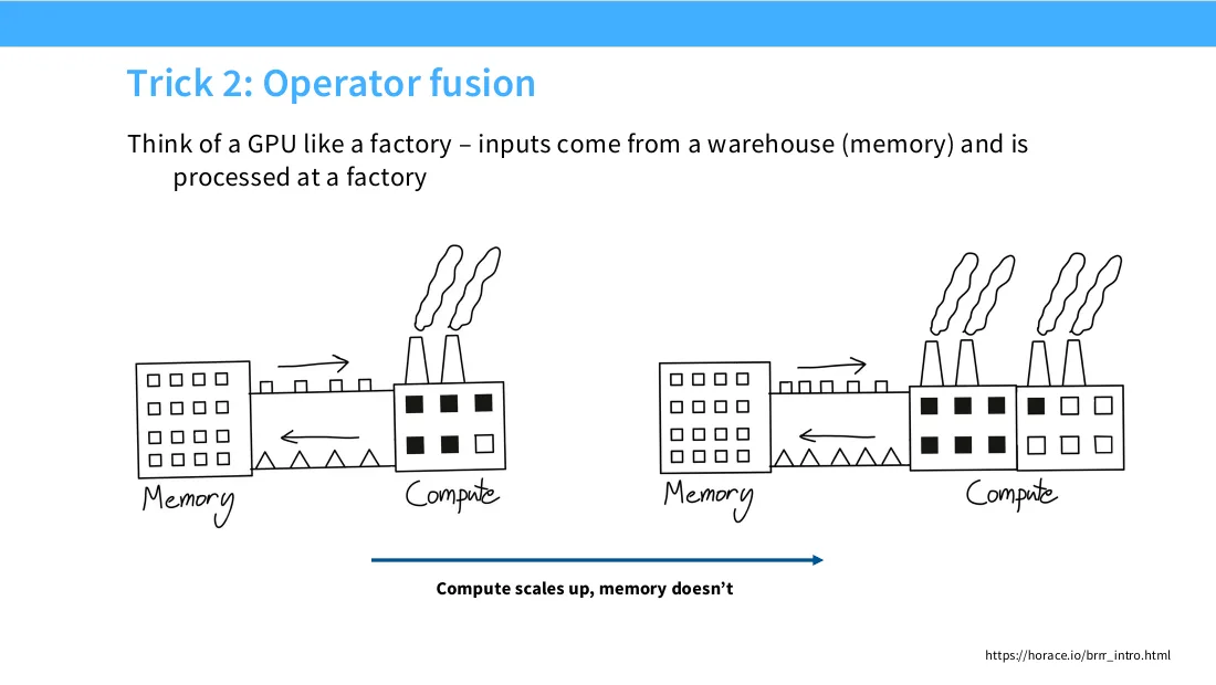
47:42 So, yeah. Okay, so the other trick, this one is much more like a conceptual programming thing, is operator fusion. It's fairly simple idea, but you'll be surprised at like, how much this doesn't already happen. So think of a GPU as a factory. You've got your memory warehouse and you've got your little compute factory. And you've got a little bell conveyor going back and forth, right? If you scale up your compute, you're going to be bottlenecked by your little bell conveyor. And this will be worse if you have many operations, right? Like imagine, I've got lots of different operations I need to do. #

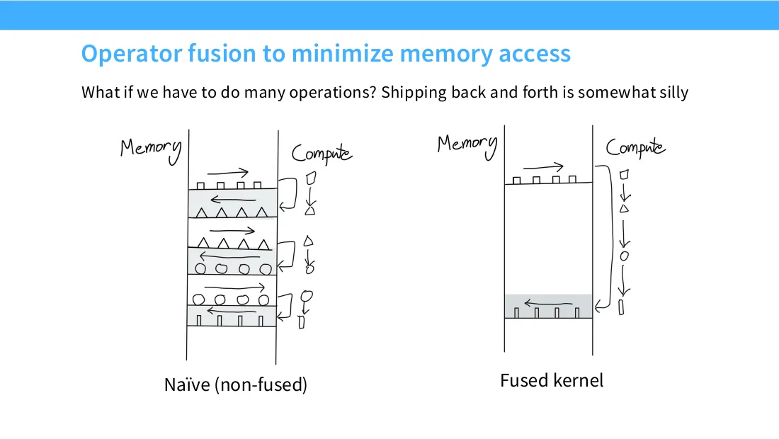
48:14 And I'm going to ship my raw materials to my factory and back and forth and back and forth. This is a lot of memory bottleneck that you're paying for, right? And lots of sort of duplex, bi-directional memory bandwidth. Now, wouldn't it be better if I just had a one giant factory that would take all the raw materials and ship back my finished products, right? This way, I only have to pay for memory bandwidth twice. Very simple idea. This is operator fusion, right? #

48:39 And this appears very often, right? If you write a very simple, let's say, computation of sine squared plus cosine squared, what does the PyTorch computation graph look like? It looks like this. You've got your x. I do my sine. I do my cosine. I square it on both sides. I add them. And I get my output, right? #

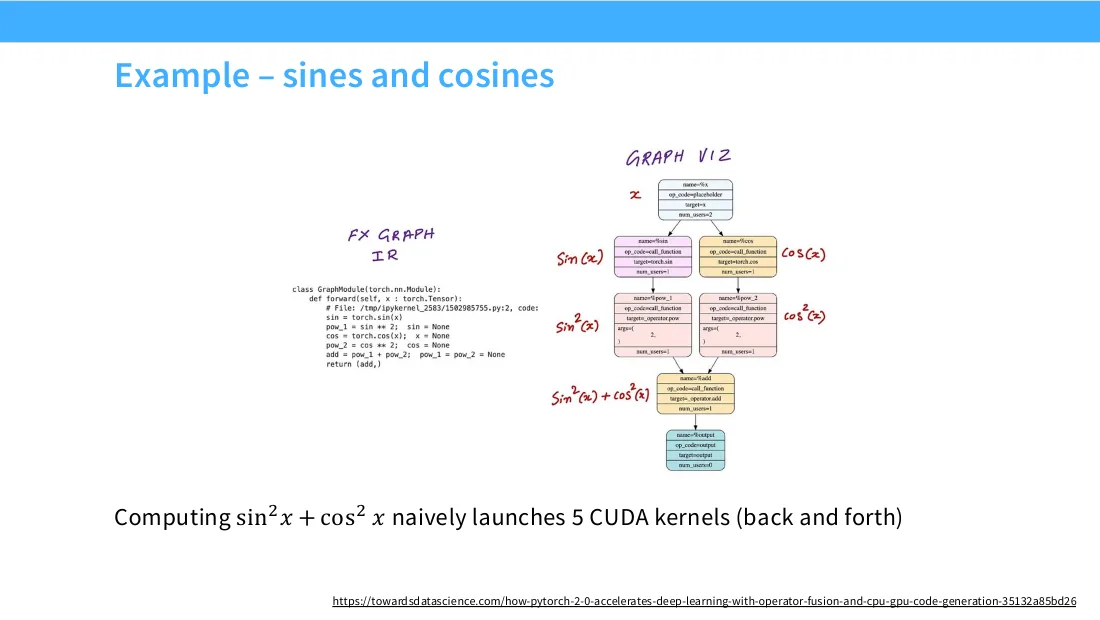
48:57 Naively, if you don't do anything smart, what this will do is each of these will be a factory, so to speak, right? You will read and write from global memory each time one of these is called, right? And you will incur quite a bit of memory cost every time you do so. So this is pretty painful. And you can imagine, instead of doing that, why don't I just write GPU code that reads once from global memory, does the whole thing, right? Inside the SM, as I talked about before. And then after it's done inside the SM, I'm going to write it back to global memory, right? A single sort of kernel that does all these operations. This is called fusion, right? #

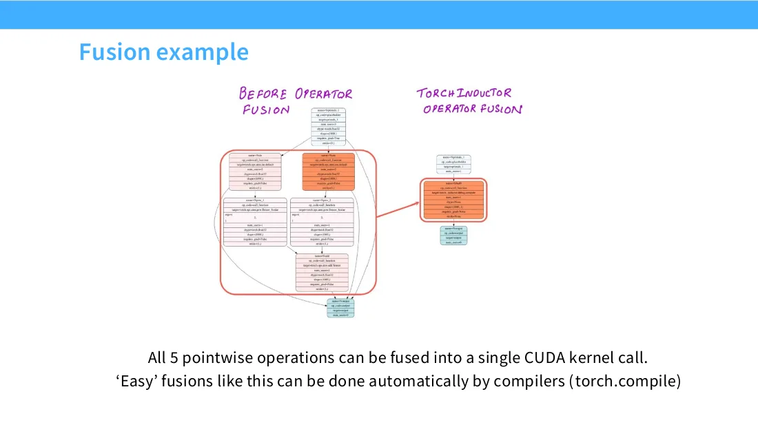
49:36 And anything that's easy like this, like this is a very easy fusion. It's like a graph that I can sort of just squish down into a single unit. A compiler can automatically do this for you. So torch compile, which is a compiler for PyTorch, or Jax compile, which is Jax's compiler, which is more deeply integrated into Jax. Both of these will fuse these kinds of basic things into a single CUDA call. #

50:01 I'll talk a little bit more about fusion later. #

10 技巧 3：重计算

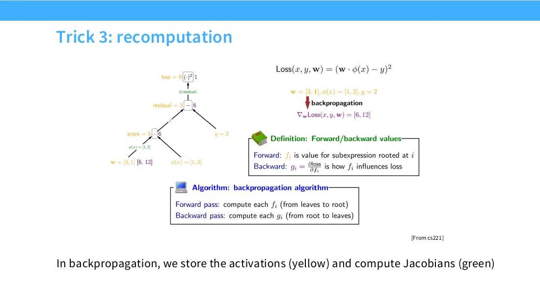
50:04 But I think this is, you know, the advanced versions sometimes require sort of manual intervention. But the simple versions you can just think of as, you know, compilation will solve your problems. Okay, the third idea is recomputation. So we know in backpropagation, what do we do? Well, we go forwards, upwards, up on the tree. This is from Percy's 221 class. You know, you go upwards on the tree, and you keep track of activations, right? You store these little activation numbers. And then when I go backwards, I'm going to use the activations that I store to compute sort of the backwards signal down my tree, right? #

50:36 We all know backprop to some extent. So, you know, we know what this is. But also, now, you know, we're looking at this not from the perspective of like mathematics, how do we compute a gradient? We're thinking about this from the perspective of systems, right? Like how do we minimize our memory? Well, if we think about what's happening, let's say I have something simple. I have x, sigmoid, sigmoid, sigmoid, out, right? Each of these sigmoids is going to generate in the computation graph some sort of residual, right? Or some sort of activation that I need to track. #

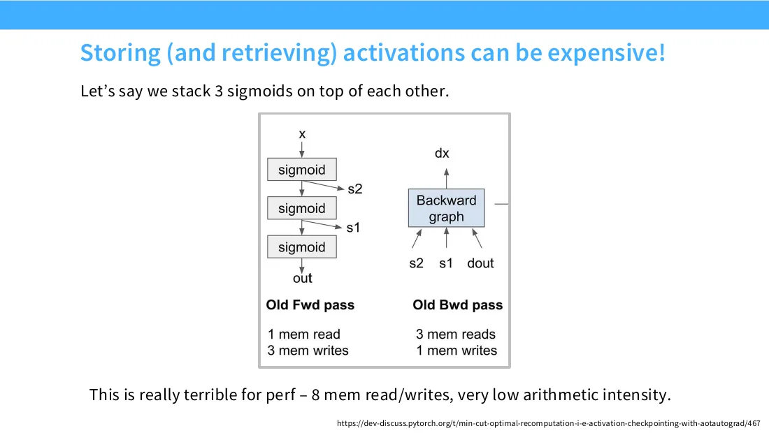
51:04 So after my first operation, I have s2, second operation, s1. And then when I need to do my backwards pass, it will consume s2, s1, and my output. Sorry, the gradient of my output. And I'm going to push this backwards towards the derivative of my input, right? So if I count the number of memory reads and writes, it's going to be one memory read for x. Three memory writes for s2, s1, out. And then on the backwards pass, this is sort of flipped, right? So this is a total of eight memory reads and writes, very low arithmetic intensity because I'm just stacking a bunch of sigmoids. #

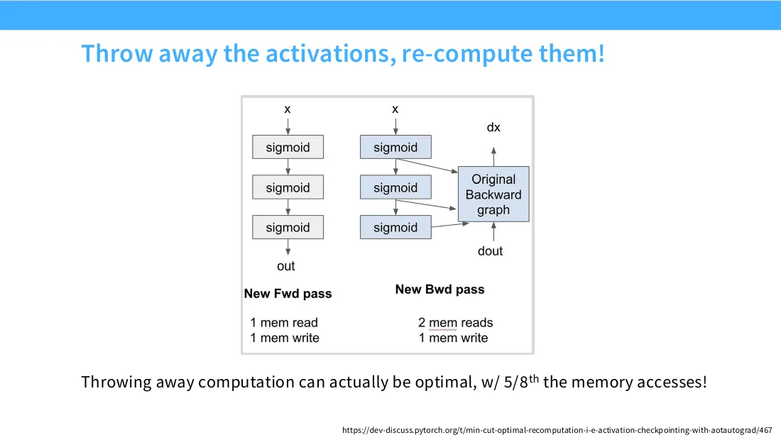
51:36 Now, what can I do instead? Well, what I can do is I can just throw away all of the activations. Normally, you wouldn't do this, right? Like why would I want to recompute something? But imagine you're in a world where computation is super, super cheap. You just have abundant computation. You're not using all of your units. But your memory is very expensive. Like any read and write has a lot of penalty. #

51:57 Then you might prefer this computation graph where I read an x and then I'm going to do sigmoid, sigmoid, sigmoid, output. I'm going to store this output. I have to write this because that's the output of my graph. But now in the backwards pass, right, my backwards graph is going to get in d out and sort of on the fly, I'm going to re-forward the x and then compute the activations on the fly right where I need them, right? So now this is going to be two memory reads for the d out and the x and one memory right for the dx, right? So I've gone from eight total memory accesses to just five, right? So now I have five eighths of total memory accesses, same computation, but I've spent a little bit of extra compute and saved a little bit of extra memory, right? This is another very important trick. We don't normally think about this because usually we're concerned with like just computing the gradient, but once you have a systems mindset, you start to think about recomputation. #

52:49 Cool. Okay. Trick number four. This is another sort of memory trivia thing, but surprisingly becomes important. And also why sometimes it's important to understand the hardware model of what you are, you're interacting with. #

53:05 So global memory, which is the big memory that lives outside the chip, is DRAM. And DRAM, because of the way that it is structured, actually comes in bursts. What that means is when I access, let's say the very first position, I don't actually get just the first value. I can read off all four of these first values for free. And that's because the way the memory cells are lined up, there's kind of these blocks of memory units, and then when I sort of activate an amplifier, I can just read out all of these almost for free, right? The way that it's sort of structured and parallel allows me to read blocks of memory. That kind of makes sense, right, as a hardware model. And so this is called a burst section. And so whenever a section is accessed, all the other locations can also get delivered for free, right? #

53:51 And you won't pay for them, so to speak. And so you might have something like 128 bytes worth of a burst. That means a single read will return potentially 128 bytes worth of data, as long as it lives in the same contiguous block. #

11 技巧 4：内存合并（coalescing）

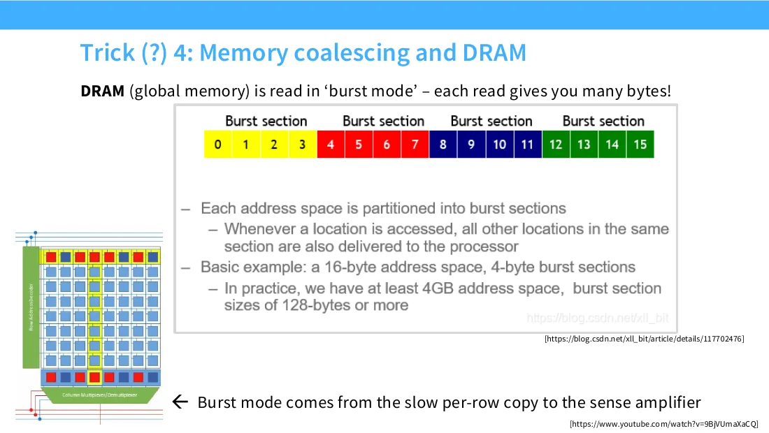
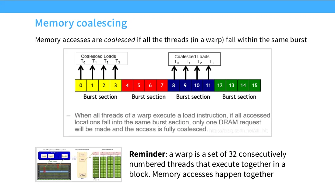
54:06 So this means that if you have your reads arranged contiguously, where they're all together, it's going to go much faster. And to use a term, you say that a memory access is coalesced. So that word means if all of the threads in a warp fall in the same burst. So what that means is, let's say I have three threads, and all three of my threads, or sorry, four threads, four threads, and my four threads live inside of a single burst section, right, or they're reading from this burst section. Then this is coalesced, right? Because they're sort of using up all of this entire burst section, and I'm fully utilizing this very nice property of DRAM memory. #

54:47 And so if I have multiple warps, I'm going to have different multiple burst sections, but you can efficiently read out of memory by sort of grouping together your memory reads. Why does, oh yeah? Sorry, this is like, why does the memory access have this, like this sort of. Which one? Like this? This one, yeah. Yeah, so as far as I understand, the memory cells are arranged in a grid, and your amplifiers for like deciding which cells to read sort of operate at a column wise level. And like activating the voltage for this is often a thing that takes a significant amount of time. So once you've like selected the column, readouts of multiple elements within that column are much comparatively cheaper. #

55:29 Is this to like select to read the upper red cell, right? Or, yeah, right. So if I want to read this, for example, right, like, you know, I'm solving this. Or maybe it's the columns that are cheap in this diagram at least. But, you know, if I'm trying to read this, I might get this whole row for free, right? Because I've addressed this whole row. Okay, so I don't get a T for free. I just- You don't get a T for free, yeah. #

55:54 Okay, good. #

55:56 Okay. So you're saying like, Tatsu, why are you telling me DRAM trivia? The reason why I'm telling you DRAM trivia is because, you know, think about matrices, right? Matrices you often want to read in big blocks, right? Because you're going to do matmoles. And certain kinds of memory accesses on matmoles are sort of privileged. They're much more nicely structured than others. And sometimes you can take advantage of this to get very, very fast memory reads. So the mnemonic or, you know, the thing that I remember is, if you have threads and you have a row-measure matrix. #

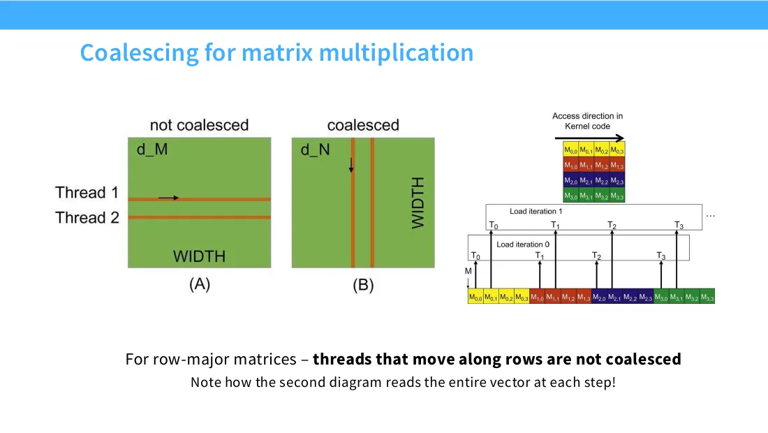
56:29 So, you know, it's sorted where, you know, each row is sort of how your indexes are increasing. Threads that move along the measure axis are not coalesced. And to really make this visual, actually, I like this diagram on the right. Imagine I have this 4 by 4 matrix where this is row-measure. So it's sorted in the order of, you know, the yellow block comes first, the red block comes next, and so on and so forth. This is the linear ordering sort of in-memory address. This is kind of the matrix that, you know, I'm trying to store. Now imagine that I have threads that are trying to read each column, each clock cycle. So I read a column, I move to the right, I read a column, I move to the right. #

57:09 If I'm doing that at the very first iteration, I hit this element, this element, this element, this element. Notice that each one of these limit a different burst window, and I read the entire vector, so to speak, right, or the entire matrix, sorry, so to speak, even though all I wanted was a single column, right? Now imagine if I was reversed, if I was flipping this matrix, I could read the entire sort of block. Every thread will get its read in a single sort of read of the memory, right? #

57:37 So coalescing can give you significant improvements in sort of reads from large contiguous structures like matrices. #

12 技巧 5：tiling（分块）

57:44 So this is one reason why you might want to think a little bit about row versus column versus other kinds of ordering. Okay. The last one that I want to talk about, and this is the big one, and maybe the most important idea, I've like saved it for last, is the idea of tiling. And I think this one has probably the big impact on performance. #

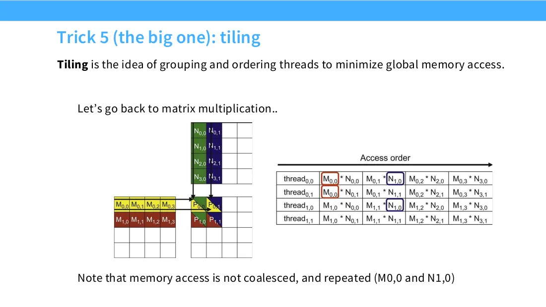
58:06 Tiling, I think, more than any other idea, is this idea of trying to do as much as you can with the memory hierarchy. So what we want to do is we want to group our memory accesses as much as possible, and sort of shared memory accesses should be done together, and they should be done on shared memory. So the reason why it's called tiling is I'm going to cut up the things that I need, I'm going to tile my space, and each tile will be loaded into my shared memory. And once that tile is loaded, I'm going to repeatedly read from that tile and do as much as I can. So let's think about the matrix multiply case. I want to multiply this matrix and this matrix, and this matrix on the right bottom, this is my output, right? This is sort of where I'm writing my matrix out. This is a pretty standard notation for this. Now, if I want to do this, right, I'm going to be reading, you know, as I'm reading through the threads, multiple, sorry, the same entry will be read multiple times. #

59:00 And to be precise, each entry will be read n times in an n by n matrix multiply, right, naively. So you might think, right, if I'm reading this entry, let's say m0 multiple times, instead of hitting global memory each time, why can't I sort of group all those memory accesses together? And the nice thing about matrices is that there's a very natural grouping, right? And this is to essentially cut the matrix up into sub matrices and then load them and then operate upon them, right? So here is a very simple algorithm. I'm going to cut up my matrices into sort of two by two, you know, sub matrices. And then I'm going to load different tiles. So I'm going to first load the m00 tile, the top left here. I'm going to load the n00 tile, the top left of my top matrix. #

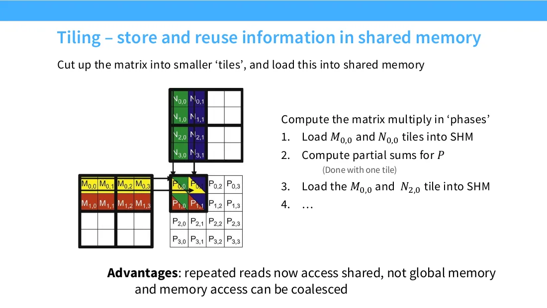
59:46 And I'm going to load those into shared memory, right? So I'm going to pay the cost of transferring those slowly from global memory once. But once they're in shared memory, I can read and write very fast with those tiles, right? This output tile will also be for now in shared memory. And I will operate on these sub matrices entirely, right? So I'll multiply these two sub matrices and I'll put the partial sum into my output sub matrix. So that allows me to do a bunch of reads and writes, all in the shared fast memory, and then I can write it back out when I'm done. What does the math look like? Well, in the non-tiled case I already told you, right, each element of my input is going to have to be read n times when I do this big n by n matrix multiply. #

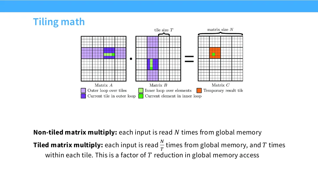
1:00:28 If I tile them with a tile size of t, then each input is going to be read n over t times from global memory, and then t times within each tile, right? And this kind of makes sense, the extreme, right? If t is equal to n, I read it once from global memory and access it n times in shared memory, right? And this is great because the t times reduction in global memory access, if you have big, big shared memory tiles, it means that you can dramatically reduce your global memory access on something like a matmul. #

1:00:58 Cool. Tiling, okay, yes? So are you doing this because you can't have the entire? Yes, yes, yes, yes, that's right. Yeah, but you know, if you were building one of these, like, very fancy alternative accelerators, like rock or something, which is all SRAM, then yeah, you just put the whole matrix in there and you're very fast for the whole thing. But very expensive, very, very expensive. Yeah? And then this also happens like. Because there's a charting, like, I gave their. #

1:01:27 So, like, and then you just keep adding that cell and then again, is that kind of how it works? You mean, like, are you asking whether this kind of, like, splitting happens at, like, the accelerator level? Yeah. That's right. That's right. That's right, yeah. So, so data parallel, you can think of as this, like, that's, you know, if I have data on this axis and weights here, if I cut it on one of the axes, that's kind of data parallel. Tensor parallel could be another kind of parallelism. All these parallels and look a little bit like tiling in some ways, yeah. #

1:01:58 Cool. Okay. Oh, yeah. So for this trick in the previous one, can I assume that, you know, a library like PyTorch will just do that in my screen? Yes, yes, yes, yeah. So, like, any, like, matmul kernel-like call will do tiling underneath. Yeah, that's right. If you're doing some sort of exotic operation, you might want to think about tiling-like things happening, right? You want to be able to locally reuse your reads. #

1:02:23 But I will say, even PyTorch or something is not perfect. And so, you know, we will talk about some of the imperfections that will happen. So tiling is very, very powerful as an idea, but it's also complex. You can actually end up with some, like, really subtle things happening with tiles. So imagine I have a tile size of 128, 128. You know, if my matrices are 256 by 256, life is good. I've got four tiles, right, perfectly cut. Now, imagine I increase my coordinate size by one, right? Now I have generated two very skinny tiles with basically nothing inside of them, right? #

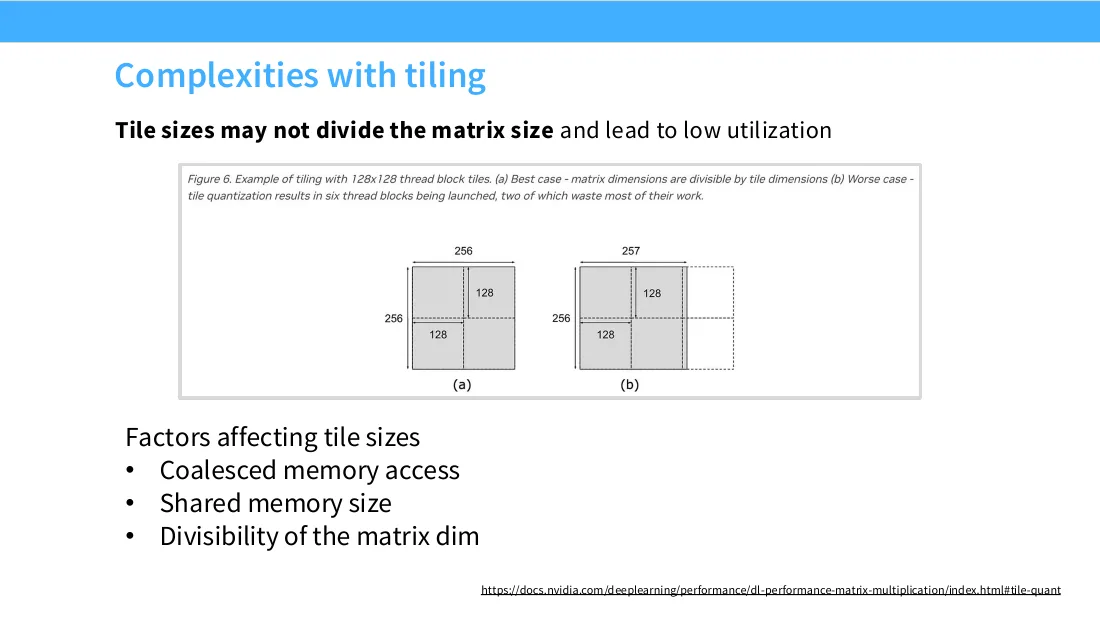
1:02:58 So now you kind of realize, you know, actually this tile sizing thing is actually pretty complex. Depending on my matrices, I might need to adjust my tile sizes to somehow, you know, trade off my memory bandwidth versus, you know, this gigantic empty space where I'm doing nothing, right? So, you know, you have to, tile sizes is actually a thing that you optimize. So like coalesced memory accesses, the size of your shared memory in your accelerator, and the size of your matrices all affect, you know, which tiles are optimal. And if you know about different options in PyTorch, you know, there's a compiler option called Max Auto-Tune. I don't know how many of you have used this or know about this. You know, you turn on that flag, for the next 15 minutes, PyTorch is going to like, you know, run an endless series of benchmarking tests. And you'll realize actually what it's doing is it's like trying all sorts of different tile sizes on your matrices and trying to figure out which one is actually faster. And you'll find that you'll get, you know, non-trivial benefits from actually optimizing these things. #

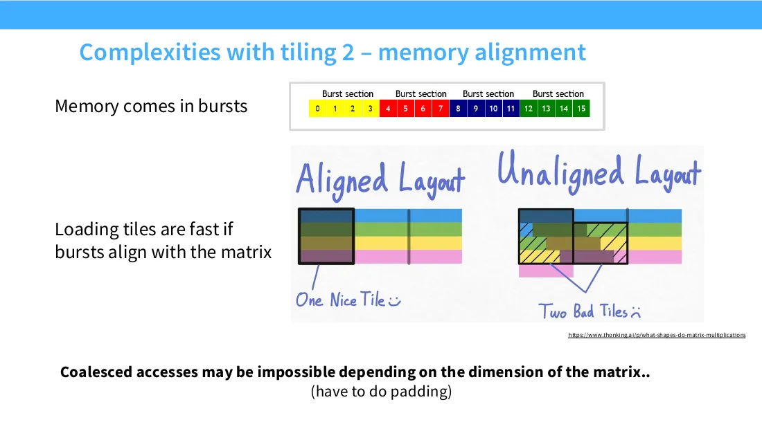
1:03:59 The other thing that you'll find related to coalescing is if your tiles or if your matrices are the wrong size, what you can do is that your attempt to read a tile might actually trigger a lot of memory reads. So imagine I have this nice world where, you know, I have, let's say this blue one is the row, and I want to read this nice tile, and my burst sections are sort of the width of the tile. In this case, if I do sort of four reads, you know, I'm good to go because of the burst sections, I've read this entire sub-matrix, right? So good memory reads from coalescing. Now, imagine I shift the matrix size by one. Now I've bumped this first row over, so this blue box now lives over here, and there's no way for me to coalesce my reads to read a single tile in one go, right? Because now all these things are sort of ragged and misaligned. So I need to do at least two tiles worth of reads to read out this one tile, right? So, you know, there's actually a lot of complexities involved in optimizing tile reads once you start thinking about coalescing and all these other things. #

1:04:59 And so, in this case, what you have to do is padding in order to line up, essentially, the boundaries of the burst sections with the tile sizes that you have. Okay. And this is why you end up getting stuff like this, which seems very mysterious. I think this is one of my favorite weird ones, right? Andre Karpathy, when he was doing nano GPT speedruns, said, well, you know, when I increase my vocab size to 50, 257 to 50, 304, you know, I got a 25% speedup, right? And it's kind of weird to have to pad in order to get a speedup, but maybe it makes sense once you realize things like this, right? Padding can start to shift the rows and columns so that you actually get very efficient reads, whereas at other times you do not. Go ahead. Is there a, is there a, you know, like tile size that you should be taking into account? #

1:05:53 You don't want to think about tile sizes per se, because tiles you should normally think of as like a lower level systems thing, unless you're writing your own kernels. But you do want to think about the size of your matrices. Okay, but you want your size of your matrices to be divisible by the tile size? You want to be, right, so you want it to be, #

13 矩阵之谜：对齐与 wave quantization

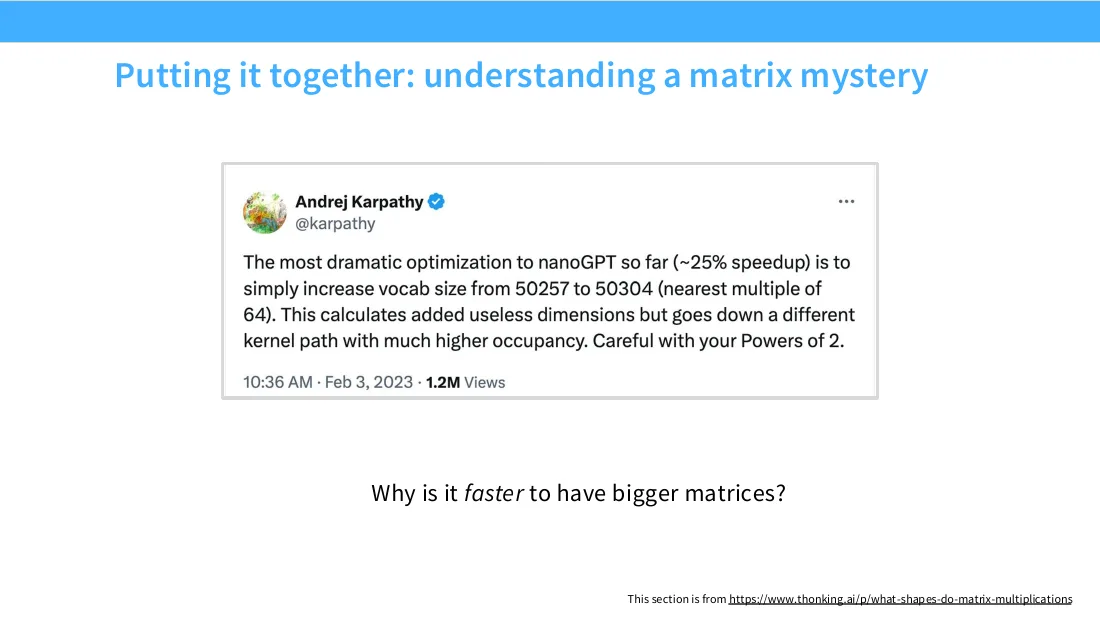
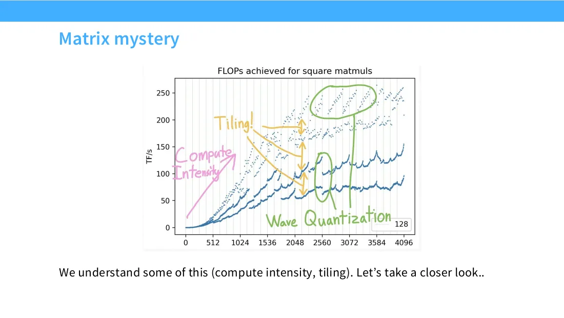
1:06:08 I'll talk about that in a moment, but right, generally powers of two, ideally divisible also by like 32, right? Okay, so now we can talk about this matrix mystery over here. We have essentially all of the pieces that we need to understand this, so we'll walk through this one by one. We've already talked about compute intensity, right? The roofline plot. You need to have enough work for each memory read in order for you to be able to saturate your compute unit. That's what's driving the sort of diagonal upward trend, so that one is done. Now let's talk about some of the other ones. First one's tiling, right? #

1:06:41 If we look at each of these lines and we color them based on essentially the, the divisibility of the matrices, you will find that, you know, the blue ones are essentially only divisible by one. They're not even, they're not even even. Yellow ones are, sorry, orange ones are divisible by two, right? Green is divisible by eight. Red is 16, and then purple is 32. And you see, you know, that the ones that are not divisible by, you know, one or just one or just two actually have very bad throughput. But once you start to get to sort of higher multiples, you start to essentially get no sort of diminishing, or sorry, no penalties, right? Like 16 or 32 perform equally well. And this is really, it's not because of like somehow powers of two are magic or something like that. #

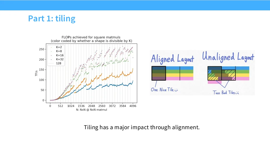
1:07:28 It's because 16 and 32 are sufficiently large that it has the right sort of burst window property. It sort of fits the whole burst window in now. And so you can get coalesced reads into your entire tile. And it has a major impact on alignment. #

1:07:42 Now, if we look at sort of what's remaining, if we look at this orange line, we'll sometimes see this weird periodic behavior where suddenly performance will drop, right? And this is very weird because I'm just multiplying matrices. Why does adding a single extra dimension suddenly kill my throughput? And this is, I think, using all the things that we learned is kind of fun to get to this end. Percy calls this GPU trivia, so I think he hates this one, but I love this one. So why is it that going from here to here, I get such a big drop in throughput? Well, it happens between 1792 to 1793. And why does this happen? Well, I'm using a tile size of 256 by 128. #

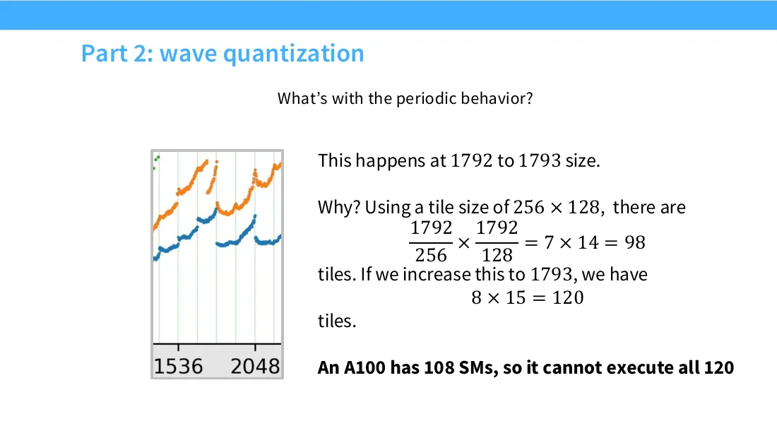
1:08:22 So that means how many tiles are there? Well, there's 98 at 1792. But once I bump myself up to 1793, well, actually, I've increased both tile sizes by one, so I now have 120 tiles. Okay, so I have 98 tiles before, and I have 120 tiles now. That's bad, but it's not this bad, right? This drop is gigantic. Well, it turns out, the reason why it's so dramatic is because the A100 has 108 SMs, right? And 98 tiles fits in 108 SMs, but 120 tiles does not fit in 108 SMs, right? And so you finish doing 108 SMs, and you're like, well, I've got 12 more of these guys, I gotta, I guess, process them, and most of your GPU is sitting idle, right? #

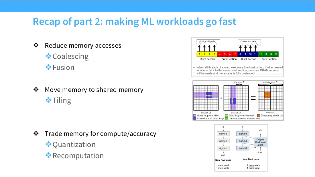
1:09:07 So you can end up with these very weird effects once again, where, you know, by bumping up your tile size by one, suddenly you need to wait a whole other cycle for you to process a bunch of tiles, right? And that's called wave quantization. Okay, so that was all for part two. How do we make machine learning workloads go fast on a GPU? Well, a lot of the story is really just about memory, memory, memory, memory, right? So how do we reduce the amount of memory access we have to do? Well, let's coalesce our memory reads together. Let's fuse our operations together so we don't have to read as much. And for the things that we have to read no matter what, well, let's reuse the memory, right? #

1:09:45 So shared memory, move things to shared memory and reuse it as much as possible, which is tiling. And then finally, maybe you can trade other resources that you have for memory, and that's quantization and recomputation, right? So all these ideas very much relate to this idea of like memories are a bottleneck. How do we deal with that, right? Cool, okay. Any questions for the last finishing? Yeah? I think we just bump up SRAM so that we can do that. Very expensive. #

1:10:14 Very energy. I mean, there's two reasons. One is it's just expensive to build SRAM. Also very difficult because it has to be physically close. Like, you know, signal propagation is hard. And I think a third reason is that SRAM and DRAM are just kind of different storage mechanisms. Like SRAM needs to be powered the whole time to hold value, very energy hungry. And so, you know, if you're thinking about total cost of ownership, energy consumption, maybe you don't want a giant SRAM chip. You really want to be using it where you need it. #

1:10:42 Yes. The whole thing scale up has like 32 or like, like, you like, operate in terms of like 64. You mean like, does it help if I go higher? Yeah. No, because I think, you know, this is really, it's kind of like, as long as it divides by your birth size, then you're good to go, right? The divisor property. There are other phenomena where you might get benefits from, you know, larger divisors, but not here. #

1:11:07 Yes. Why 108? #

1:11:10 That's just the number of SMs. You will have to ask Jensen for that. I do not have an answer for you. Yes. So, you're going back to the, to the hardware side, sorry. Not this, but, I, it just occurred in my mind. Have you started, GPU, versus, C-U-P-Rass's wafer scale angle? Yeah. I mean, I think sitting over there knows much more about wafer scale stuff than I do. #

1:11:36 We were, we were talking about last, after last lecture, how difficult the compilation was. Because if you have something wafer scale, then you have like, wave interference effects and all sorts of horrible things that happen. That's a world that I'm not familiar with, but I think is much more complicated #

14 Part 3：用这些知识理解 FlashAttention

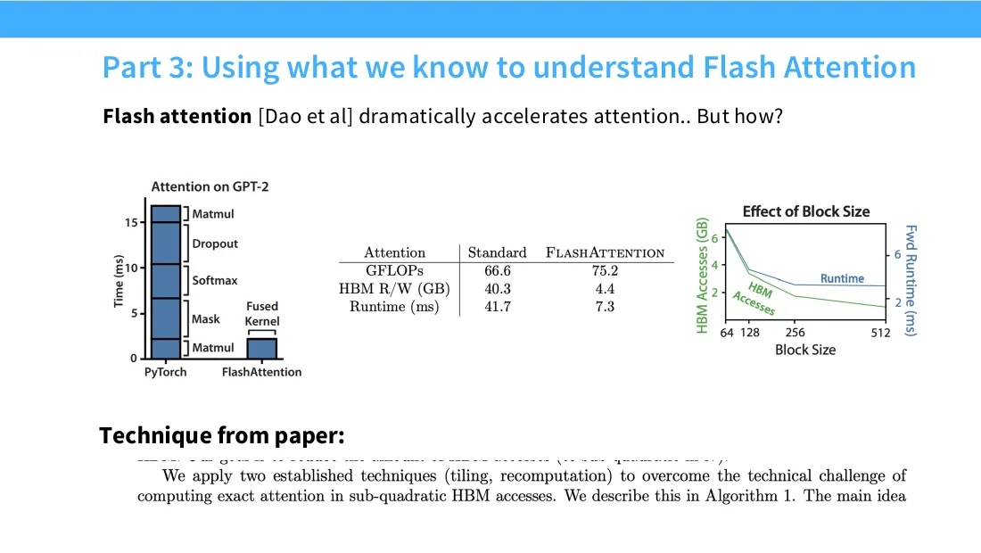
1:11:49 than what we have here. Okay, cool. All right, so now I think we can talk about, in some sense, the finale. which is, we've learned a bunch of things about GPUs. It would be nice if we can tie that all together to essentially be able to reproduce or understand something that I think is really important in advance, which is flash attention, okay? So flash attention is one of the big, I think, improvements in attention capabilities in a while. And it's all systems, right? So it's going from just PyTorch's naive implementation of attention to a single, very cleverly fused kernel. You know, this is from the original paper, but you've got this dramatic improvement in the latency of serving these things. #

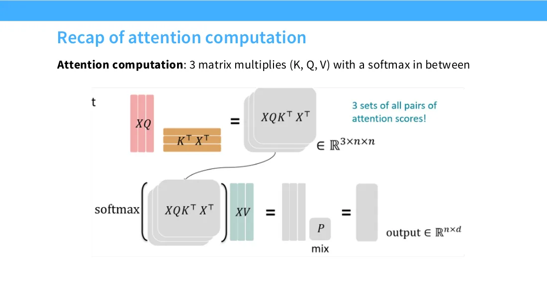
1:12:27 And as I showed you in, I think, two lectures ago, right, flash attention is, is a nice memory efficient way of computing things. So you can do bigger and bigger attention. And you can see, you know, a lot of the gains are going to come from, improvements in the amount of memory that is transferred from HBM, which is the, the global memory, right? Okay, so what, what do they actually do? If you read the paper, you know, they'll say, okay, we, we just do two things. We apply tiling and recomputation, right? And then we do it in a way that allows us to do things sub-quadratically in the number of memory accesses. I think we understand all of those components now, so let's see what's actually happening. So, remember attention computation, right, has, a couple of things. #

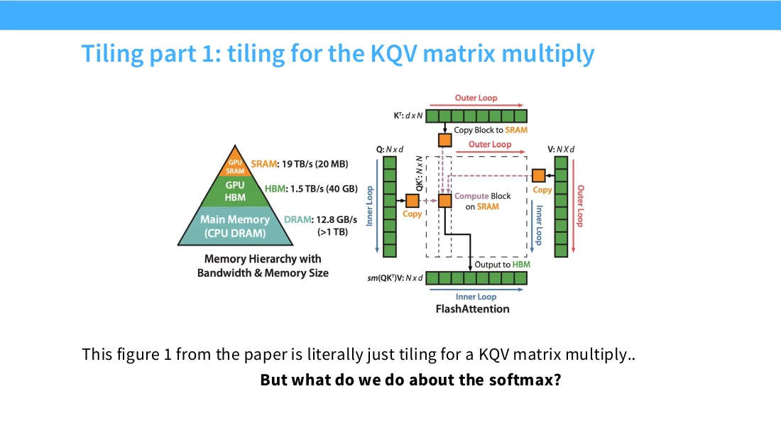
1:13:09 It has a KQV, and we do a, you know, multiple, matrix multiply with the Ks and the Qs, and then we have a matrix multiply with a V at the end, and I have a softmax in the middle, right? So those are the operations that we need to deal with. Three matrix multiplies and one softmax. So, we have matrix multiplies, we know how to do them now, right? So we're going to do a tiled matrix multiply. Figure one from the paper is literally just tiled matrix multiplies, right? We've seen this before. We're taking our inputs, our Ks and Qs, we're cutting them up, and we're just multiplying them sort of chunk by chunk on a tile. And then after we do the computation, we write them out. #

1:13:44 Nothing fancy or special here. The thing that is tricky about flash attention, and you'll see this in the assignment, is there's a big global softmax on the whole thing, right? So we can't just do this naively, because the softmax is a global operation that ties everyone together, right? So it connects all the different tiles together. It might not seem obvious how to tile attention. The key trick, and once you see this, this is really the core, I guess, idea or observation. Once you see this, the rest is very simple. Normally, to compute a softmax, you would do it kind of this way, as shown in this plot here, which is you would exponentiate all of your elements, you would subtract the maximum for numerical stability reasons, and then you would normalize that, right? Standard softmax. #

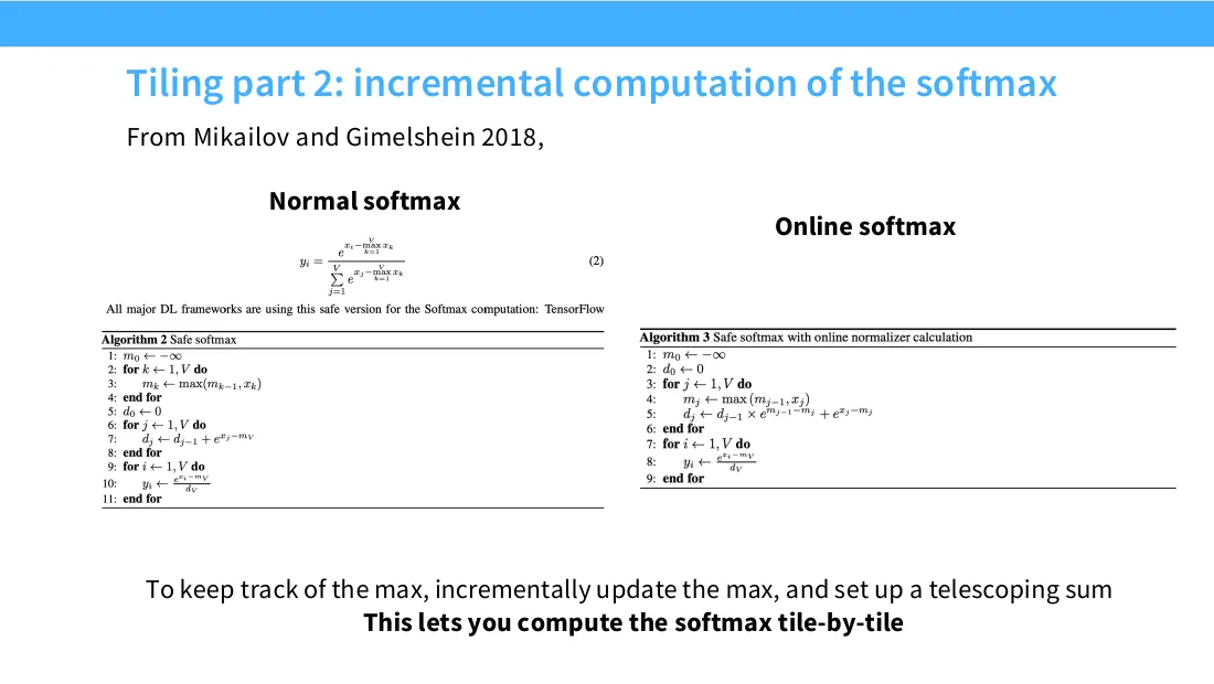
1:14:28 Now, there's a different way of computing this online, and I think once you sort of realize it, it's kind of simple, which is you're going to sort of, as you go, compute the normalized softmax. And every time you encounter a bigger number than what you've seen before, you're going to sort of swap out the maximum, right? And so you have an online way of computing sort of the softmax as you go. The only tricky thing, of course, being the max, and the way we deal with the max is we keep track of the max, and then we sort of swap it out and correct for it every time we see a new maximum. Otherwise, this is really just the online running sum of an exponential from everything that we've seen before. And of course, at the end, you'll just divide everything by the accumulator that you've computed online. Now, the important thing about the online softmax is because it's online and it goes kind of block by block, or piece by piece, we can compute this tile by tile, right? I don't need to see the rest of the tiles in order to compute this. So I can compute the softmax for my tile, and then I can sort of save the partial results, maybe write them back to global memory, and then just sort of continue on with my day. #

1:15:28 So this allows us to now break up sort of all the different interacting pieces into something simpler. So this, I think, is a, I think this was from flash attention two or maybe three. I think it's two. I like this visualization, which shows you, you know, which parts are being tiled. So the dashed blocks are being done, tiled in SRAM. The blue boxes are the ones that are in high bandwidth memory, the global memory. And what you see is, let's say we do the KQ, you know, inner product. You know, these are tiled matrix multiplies, and they're stored in SRAM. And we keep them in the SRAM, and we compute this exponential. #

1:16:04 And then similarly, in this tile, we're going to compute this running softmax. And I'm going to move to my next tile, and I'm going to do the same thing. But now I'm going to keep sort of the partial running sums of my softmax as I go. I can keep them sort of in shared memory or in registers or elsewhere. This is a very small number of things to keep track of. At the end, after I've computed all these exponentiated quantities and my normalizers, it's very simple to just multiply it with a V, once again, at the tiled form, and then divide at the very end, right? This allows me to essentially take the attention operation, cut it up into these small tiled chunks, and then go. #

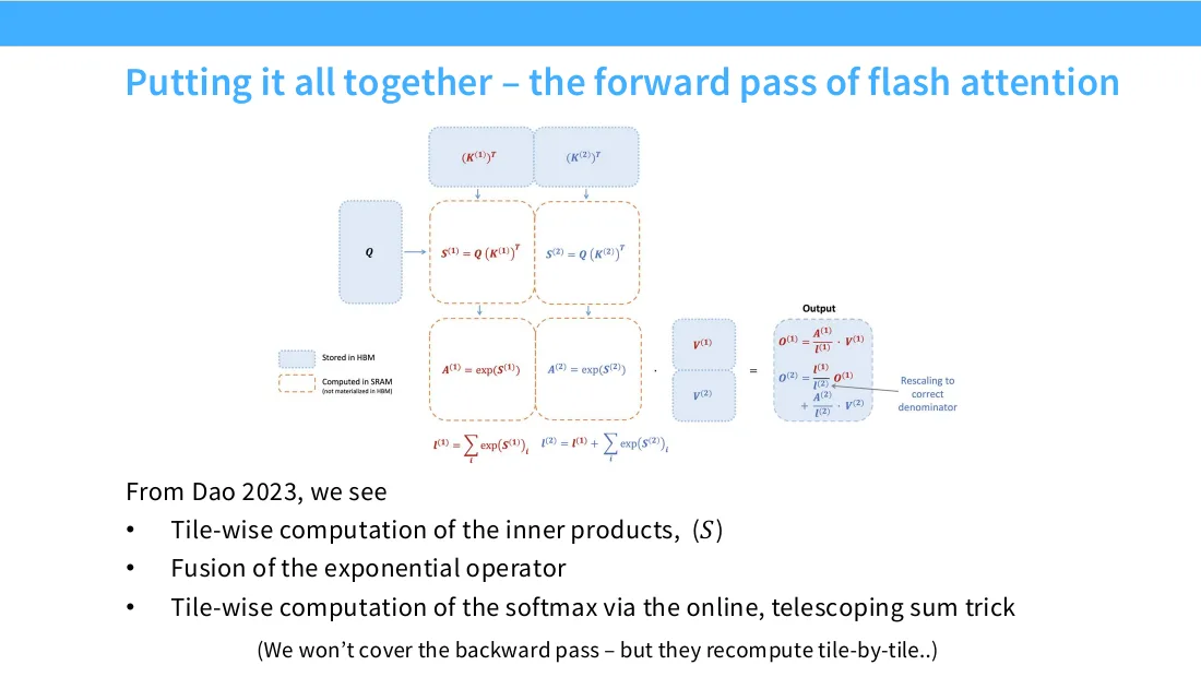
1:16:42 Finally, you've got fusion. You're going to do both of these together, right, as much as you can without going back and forth. And then, I'm not going to cover this or talk about it, but what you can do is you can, in the backward pass, recompute everything that you need, right? So the last piece of flash attention is if you saved your activations, you still have this n squared sized activation that you're going to need to save for your attention. Instead of saving that, throw it all away and recompute everything tile by tile on the backward pass, right? So it's got the recomputation piece as well. Okay, that gives you flash attention. Now, we've seen all the different tricks in action, and that's essentially all there is, right? A lot of the tricks that you see for efficient implementation and how to use GPUs well boil down to those kinds of ideas. #

1:17:28 So to put it all back together, right, important to understand the hardware. The hardware, in our case the GPU, is powering scale and compute, and we need to understand, really, all the way to the low level details to fully grasp why we make certain decisions. #

15 全课总结

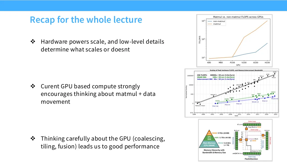
1:17:43 Like, I think, you know, I don't want you guys to be the kind of people that cargo cult, you know, 32 multipliers for your matrices. I want you to really understand, you know, why we do those things. And that goes all the way down, in my opinion, to the hardware level. The other thing is that, you know, the current, you know, way that compute is growing means that we really want to think about matmuls. Those are the core operations that are very arithmetically dense. And because of the gap between compute and memory, we need to think very carefully about data movement, right? And then finally, things like flash attention, I think, are really cool. There's also, like, architecture work that's, like, very hardware aware. Thinking carefully about the hardware when we do things like architecture design is, you know, critical to good performance for future systems. #

1:18:28 Thanks. #

1:18:37 Thanks. Thanks. Thanks. Thanks. Thanks. Thanks. #