架构与超参数

01 引入：从原版 Transformer 到你实现的现代变体

0:05 So today we're going to talk about architecture, which at least to me has always been pretty inscrutable. And so I'm going to take the approach of just telling you kind of everything, right? I'm going to go through all of the modern papers, and we're going to just look through what has everyone done. And so I've titled this everything you didn't want to know about architectures and hyperparameters, because I think we all wished we lived in a world where the only things you had to know were like VC dimension or something, right? Like very simple theoretical tools, but that's not really where we are. So, okay, what we are going to do is we are going to try to understand architecture from kind of like a survey lens, right? The best thing to do, better than listening to this lecture even, is for you to go out and train your own models and try different architectures, right? That's by far the best thing to do. That's part of the philosophy of the course. #

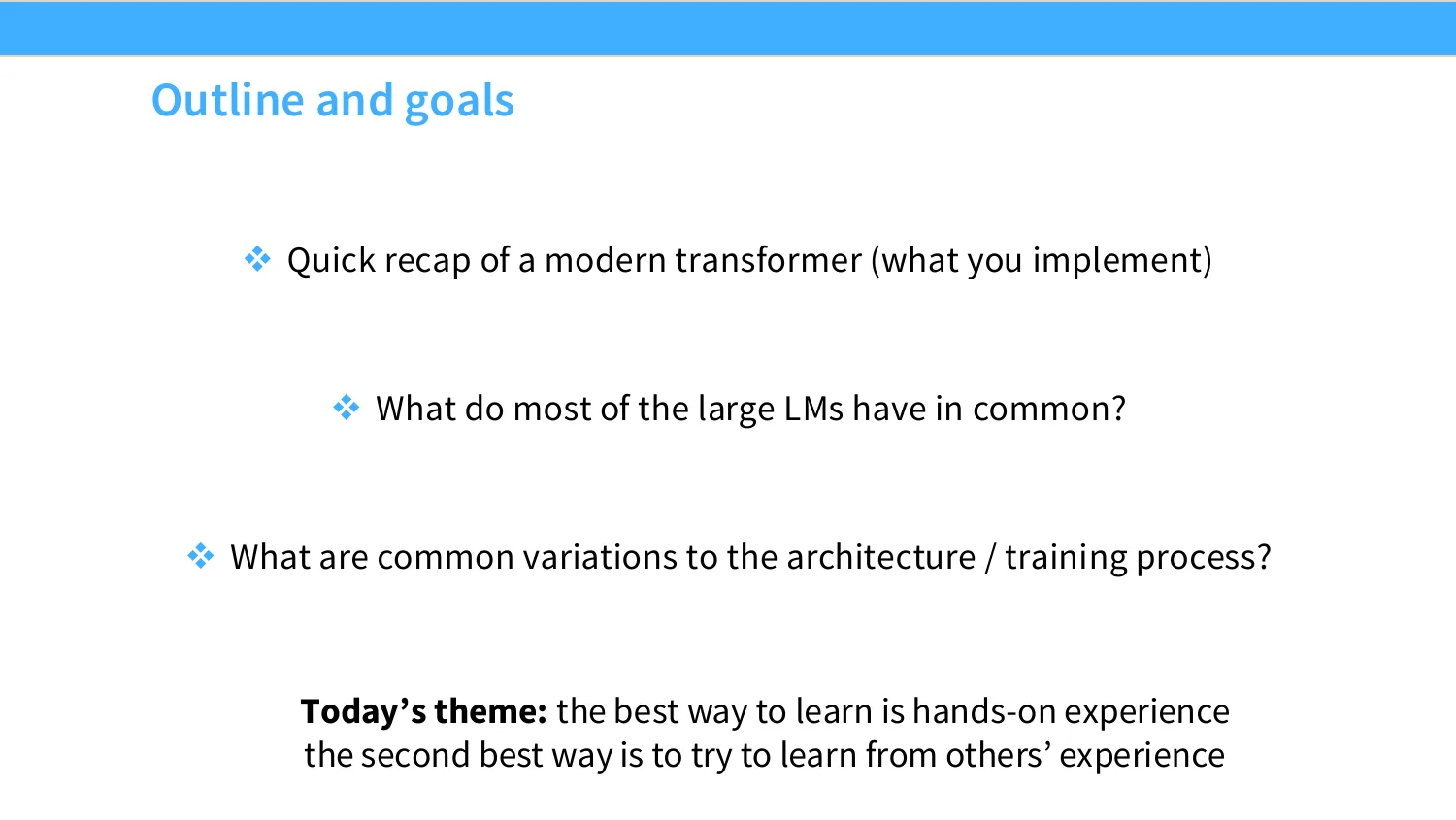
0:55 But we're not going to be able to cover the whole design space of all the different architectures that are out there, right? Like that's not something that we have to compute or the time to do. So my opinion is the second best thing that we could do is to try to learn from the experience of others, right? What has everyone else done? What are the choices that they are making, right? And by looking at kind of a broader, somewhat zoomed out picture, maybe we can start to understand, oh, these are the kinds of parameters and choices that are sort of fixed across all effective architectures. And these other ones can be sort of varied without impacting how the model will perform, right? So I'm going to talk about, you know, basically transformer variants. Like what is the, you know, modern transformer starting with, you know, the Vaswani paper. #

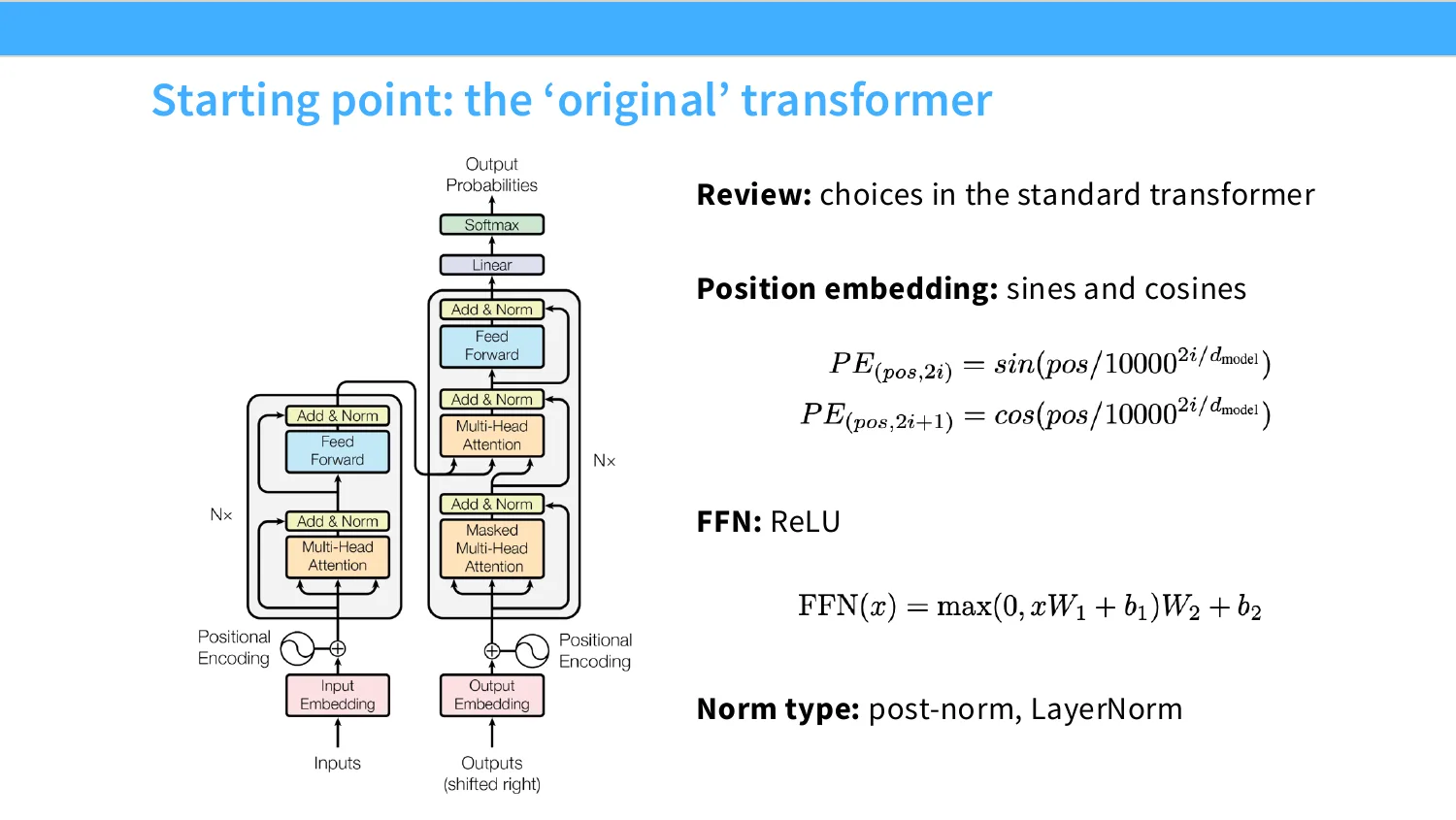
1:37 And then, you know, as we go to more modern, more recent architectures, what do they have in common? And then what are we allowed to vary? Or not allowed, but what do people vary as they go through this, right? So I think many of you have taken an NLP course of some kind, or at least seen a transformer. So you've probably seen, you know, the very vanilla transformer from Vaswani at all. You know, there, there are some fairly standard choices that you make. You say, oh, transformers don't have positional dependence, so we're going to add a position embedding. And what do we do? We're going to add some sines and cosines. #

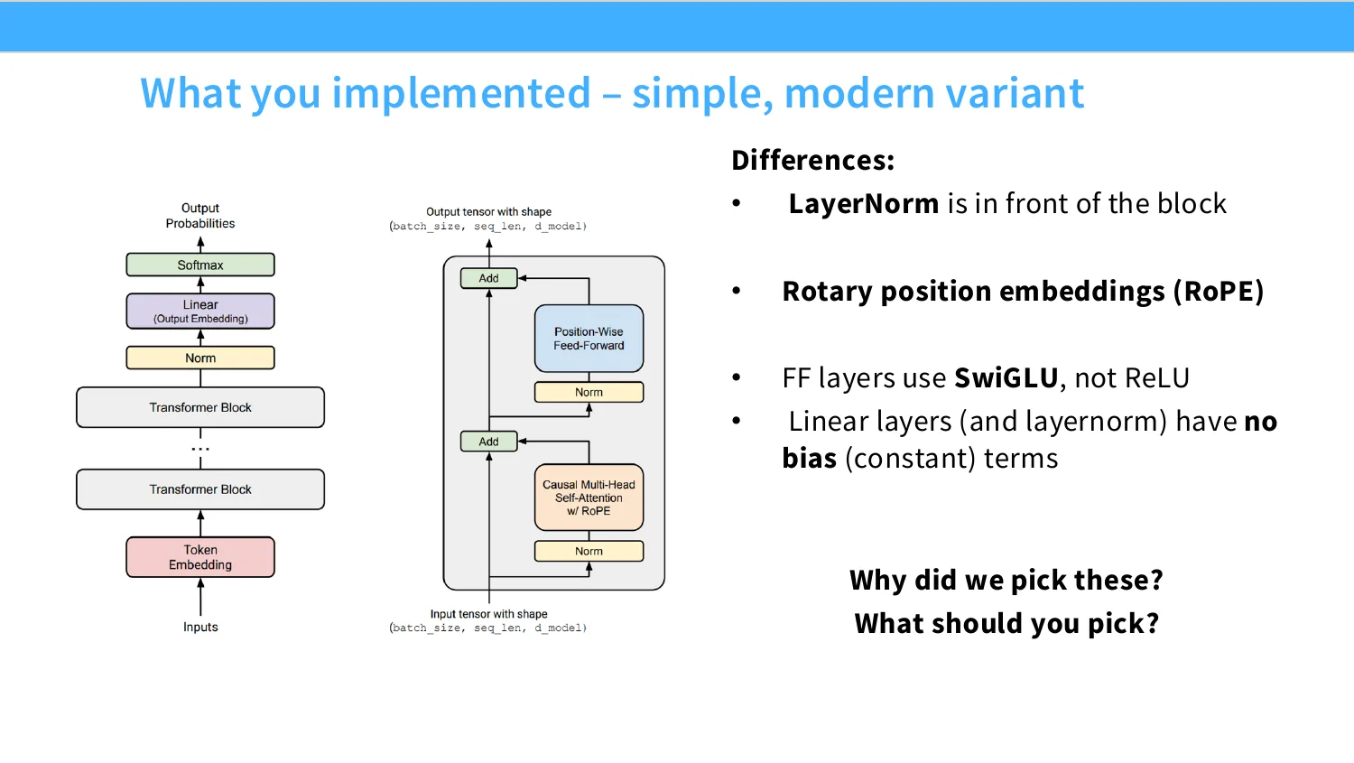
2:11 We're going to have information processing through relu. And then we're going to have a post-norm. I'll talk about what exactly that is later. And when you look at your assignment, your A1, you're going to notice some differences between the standard or the vanilla transformer and what we've asked you to implement. Well, we're going to ask you to move the layer norm to the front of each transformer block, or the non-residual layers. We're going to ask you to implement something called rope. And we're going to ask you to implement something called swigloo and not relu. Right? Why do we pick these? #

2:43 One reason is we've copied a lot of this over from Lama, but so did everyone else. Really, I think if you were to train on your own language model, I think you'll quickly run into this question of, oh, there's so many choices. #

02 如何思考架构：数据驱动的全景

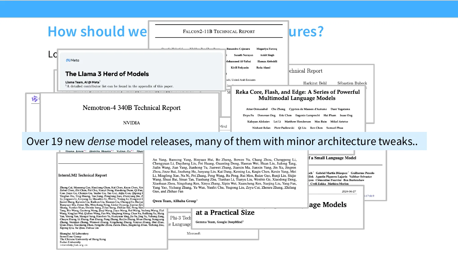
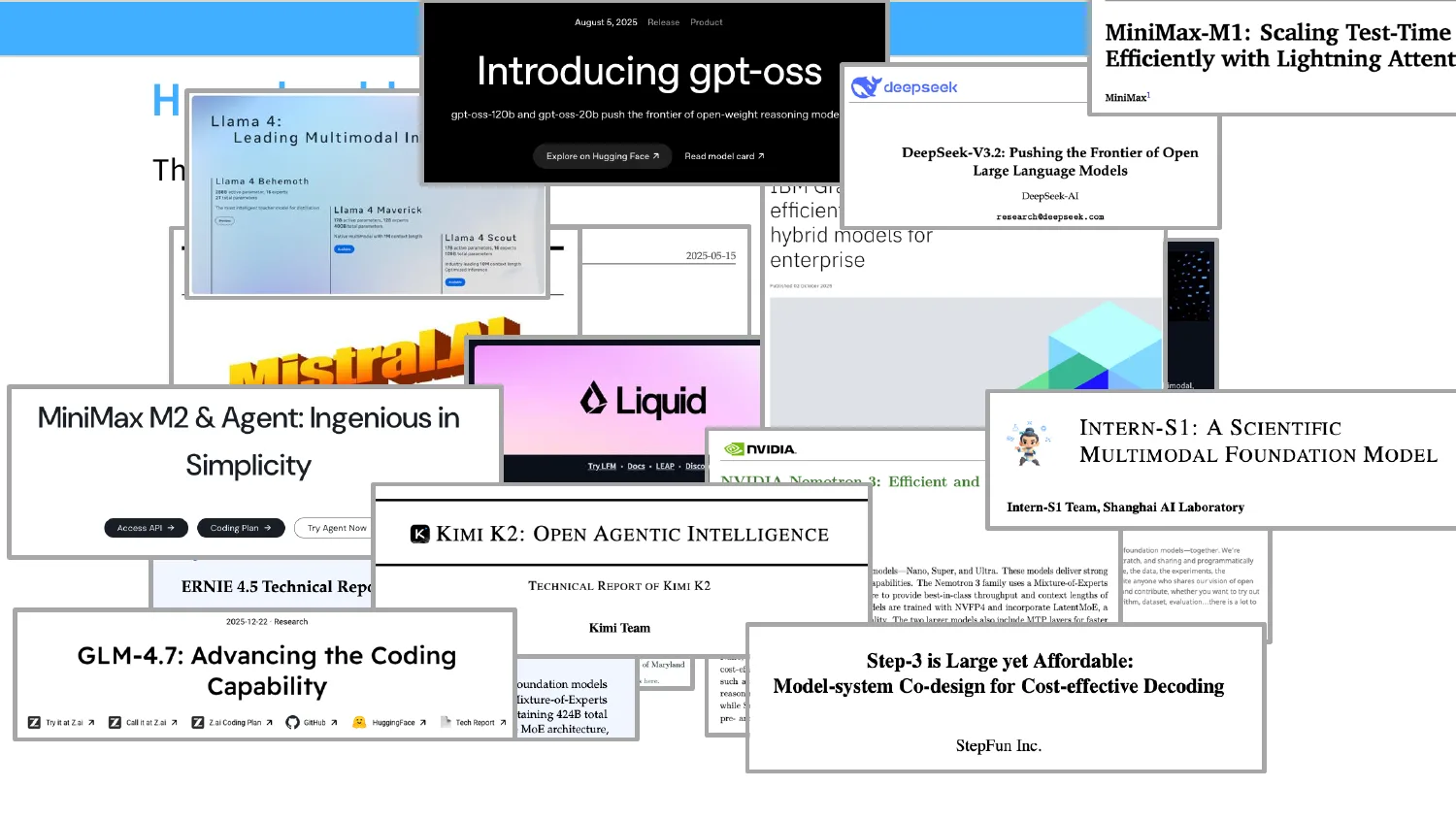
2:54 Right? Like, what do I choose for all these things? And so let's now sort of walk through all these different models. The way I kind of think about architectures is to think about, to look at all the different things people have done and say, what are the things that people have done? Can we pick and choose from those? Percy always makes fun of me for this a little bit, but I try to look at all the different models that come out each year to try to make this lecture. And last year, I thought, oh, there's just a couple papers. It's going to be fine. It's going to be fine. #

3:23 And then I look through all the things, and there's a lot of papers. There's Quint 2 and Gamma 3 and Intern LM 2. And then there were even more. There's like Nemo Tron 4 and Quint 2. And oh, oh my goodness, there were 19 new dense models. And so last year, I had my work cut out for me. And then this year, you know, I thought, well, there can't be that many new LM releases. Like, it's got to be slowing down, right? Like, people can't keep training 20 dense LMs per year. #

3:47 That's technically right. There aren't as many dense LMs. Initially, you know, I was like, oh, there's Quint 3. Gamma 4 just came out last Thursday, so I put that in there. And Olmo 3. You know, there's only a couple. And of course, I have to give a shout out to Percy's own 8B model, trained with Marin. And I was like, oh, we'll just have a few things to cover. But it turns out, if you start looking, there's a lot of different models. #

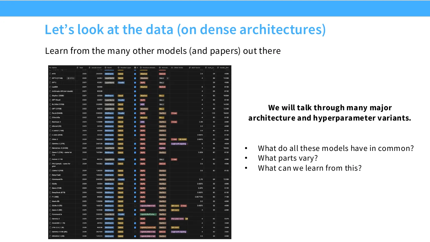
4:07 And so the fact that we have so many different models, most of these actually are MOEs, mixtures of experts. And I'll be talking about that tomorrow rather than today. Because we have such a big diversity of models, we actually get a pretty good picture of all the different choices that we can make. So I made this, like, little table. We'll come back to this little table at the end of the lecture. But basically, at this point, you know, starting with, you know, the original transformer, there's been actually quite a few autoregressive language models kind of trained on the same class of things. And you can ask questions like, what are the different vocabulary sizes? Or what kind of layer norms do we use? Or, you know, what kind of position embeddings do people use? #

4:49 And we see some fairly clear trends. I'll be talking about this as we go. Okay. #

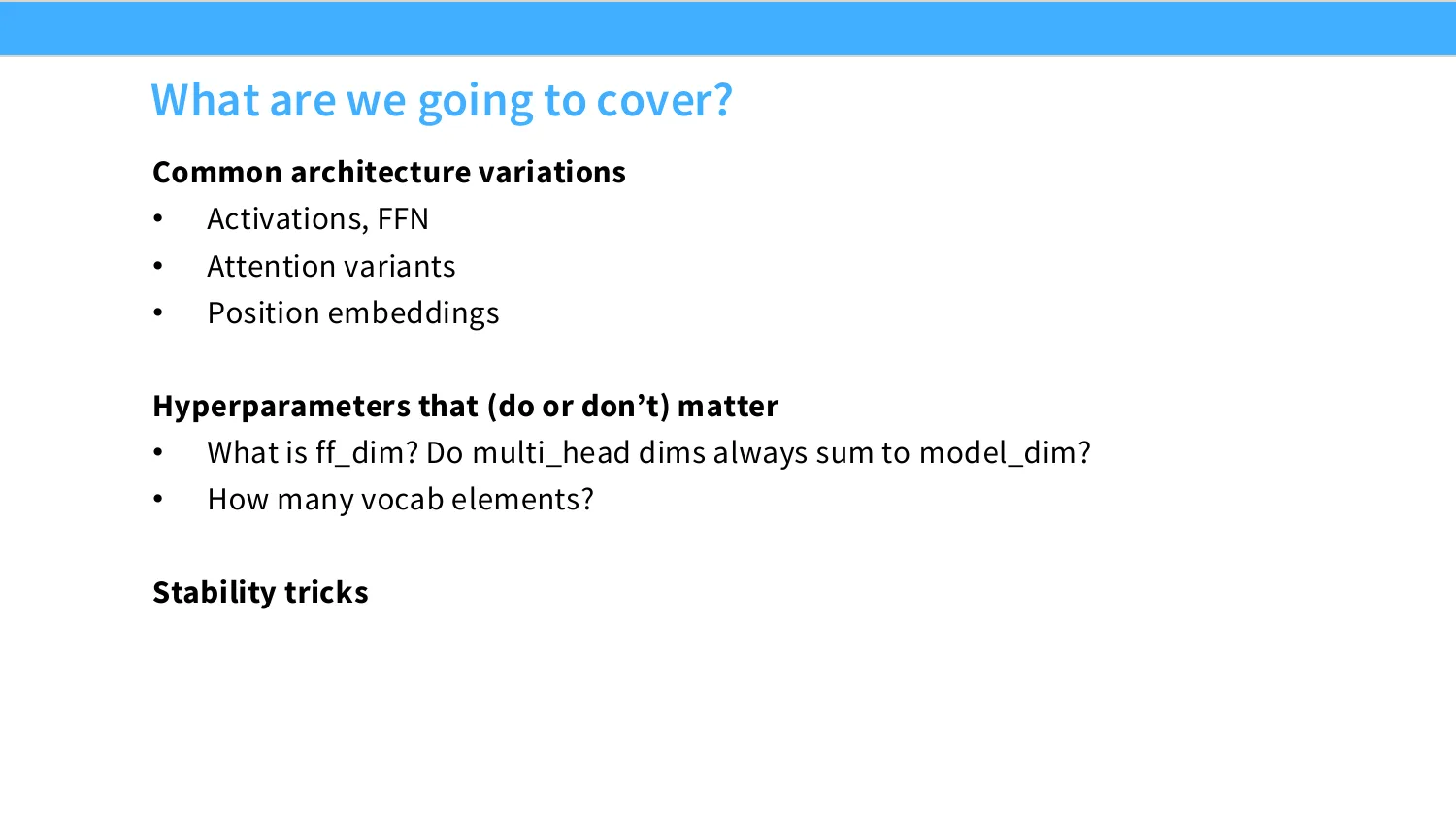
4:56 So the goal here is that we're going to cover a couple different things. We're going to cover common architecture variations. So these are different building blocks of the transformer. And after we've established what the standard building blocks are, like, you know, what do we use for the non-linearities? Or what do we use for position embeddings? Then we're going to talk about hyperparameters. We're going to go down even lower detail and say, like, you know, what is FFDIM? Should we make that a multiple of four? Or, like, multiply the hidden by four to get FFDIM? #

5:25 How many vocab elements should I have? And then after that, we're going to talk about very low level tricks of how to get models to train stably. And the reason why I'm going to talk about that in this lecture is because these stability tricks have a pretty close connection with the architecture variation, right? One of the things that, you know, higher level I want to sort of impress upon you is the architectures are actually a very complex set of trade-offs, right? Like, what does an architecture have to do? Well, it has to learn from data. So it has to generalize. It has to train efficiently on GPUs. And it has to not blow up, right? #

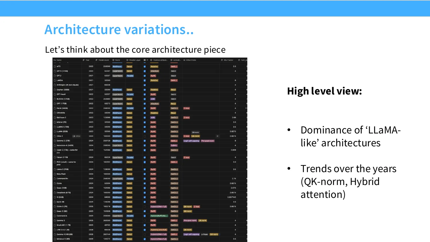
6:00 Like, halfway through training, if you're, you know, training losses just go, like, down like this, and then suddenly blow up, that's no good at all, right? So all these different requirements end up getting baked straight into the architecture. And that's why these things are a little bit messy and a little bit complex. But you should keep that in mind, and that's why, you know, things are in many ways not so elegant. Okay. So we're going to start with the core architecture piece. And as a high level view, you know, I think the way that I see a lot of the architecture stuff, you know, looking basically historically, is kind of in the early days of, you know, starting with a transformer until, you know, GPT-3 or so, there's a lot of experimentation that happens. People try lots of different things. There's no, like, gold standard that everyone has unified on. #

6:45 And then, you know, LAMA-2 comes out, and everyone's like, wow, LAMA-2 is great. I want my own LAMA-2. And so everyone starts training LAMA-2 alikes with, you know, minor variation that people have. And then finally, you know, last year, we saw really big differences or sort of a trend towards architecture modifications that make training more stable. And this year, we see lots of trends towards architecture variations that enable longer context dependence. So there are these big themes that are happening, but really I think, you know, you see this, like, big point when LAMA-2 comes out and everyone's like, wow, I want to train some of that. And then suddenly, or not suddenly, but after that, people are starting to explore once again. So it's kind of cool to see all of these different changes. #

03 归一化：Pre/Post-norm 与 RMSNorm

7:29 Okay. I think people can disagree about a lot of things on architectures, but there is one thing that everyone agrees on. You know, like, if you take the transformer paper, I think a lot of people say, like, the transformer people got, like, most of the things right, except this. And the thing that they really did not get right, or, like, I think most people agree they did not get right, is where you put the layer norm. Right? So in the original transformer paper, you know, the layer norm goes in what you would call the residual path. Right? So in the transformer, you know, you have the residual stream, this X that kind of runs through the whole network. And then you are going to be applying attention, which, you know, does some computation, and it will add back sort of a delta back into this residual stream. #

8:15 And then in order to make sure that these gradients are sort of stable across layers, you know, a layer norm is placed at the end of each of these components. #

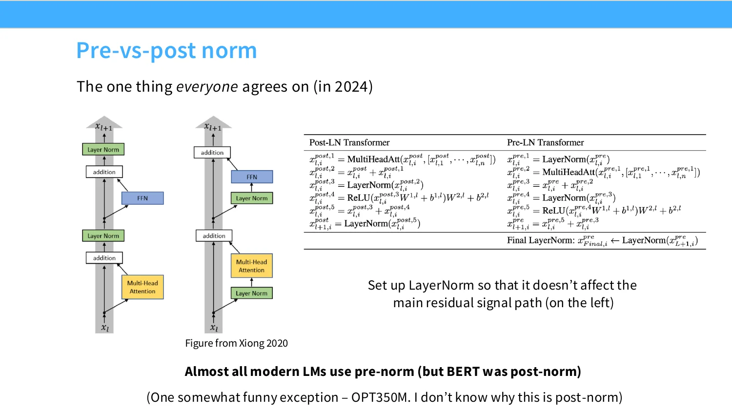
8:26 Now, instead of putting the layer norms in the residual stream, there's an alternative. I'll refer to this as pre-norm, in which you can put the layer norm outside of the residual stream, but before each of the computations. So you can put it before the multi-head attention, you can put it before the FFN, right? We'll call this pre-norm. The nomenclature will get a little bit confusing. You can call this post-norm for now, but let's call this sort of residual norm, right? Because you're putting the norm in the residual layer. Basically, all modern language models push the layer norm outside of the residual stream. This is just like a thing that basically everybody does. #

9:07 There is one funny exception, but it is OPT350M, and if you all are familiar with sort of language models, we kind of know OPT in general was kind of a mess of a language model, right? And OPT350M is even more so, because I don't know why only that model has a post-layer norm in the residual stream. OK, so this is one of the things that everyone agrees on, and so you might wonder, why is this such a unified thing across all the different models? So this is a very interesting model. And if you look at some of the early works studying, like, where do you place the layer norm style research, what you really see is that, you know, the early motivation for a lot of this was when you train a transformer, you need to do a warmup. Actually, you know, modern transformer training still does warmup as well. But you definitely need to do warmup when you train. Now, wouldn't it be nice if we could remove the warmup, right? So that was kind of the initial motivation for a lot of this research. But people quickly realized that removing the warmup #

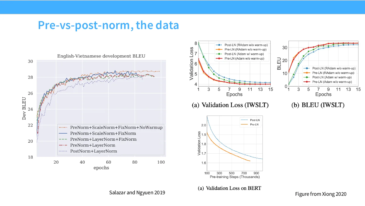
10:14 had very serious issues in terms of the stability and convergence of these things, right? So if you did post-norm plus layer norm, which is, you know, basically the original transformer thing, you got this purple dashed line, oh, you just don't converge as well, compared to doing something like pre-norm, you can ignore the other terms, you would get much nicer convergence even without warmup, right? So this was the original motivation. But really what people kind of quickly realized is that, you know, moving the layer norms outside the residual stream has some pretty important implications as you make your network deeper and as you start to grapple with stability issues. To me, I think the gradient attenuation issues are kind of the most clear. When you sort of talk to people who do architecture design, I'm not really one of the people that deeply engages in this, but one of the things that people often say is keep your residual stream clean, right? So in this case, you have your x's coming in from the bottom on the pre-norm side, and this x propagates all the way up to the top, right? All the way up to your final output. And that allows gradients to propagate in the backward pass straight through this, right? #

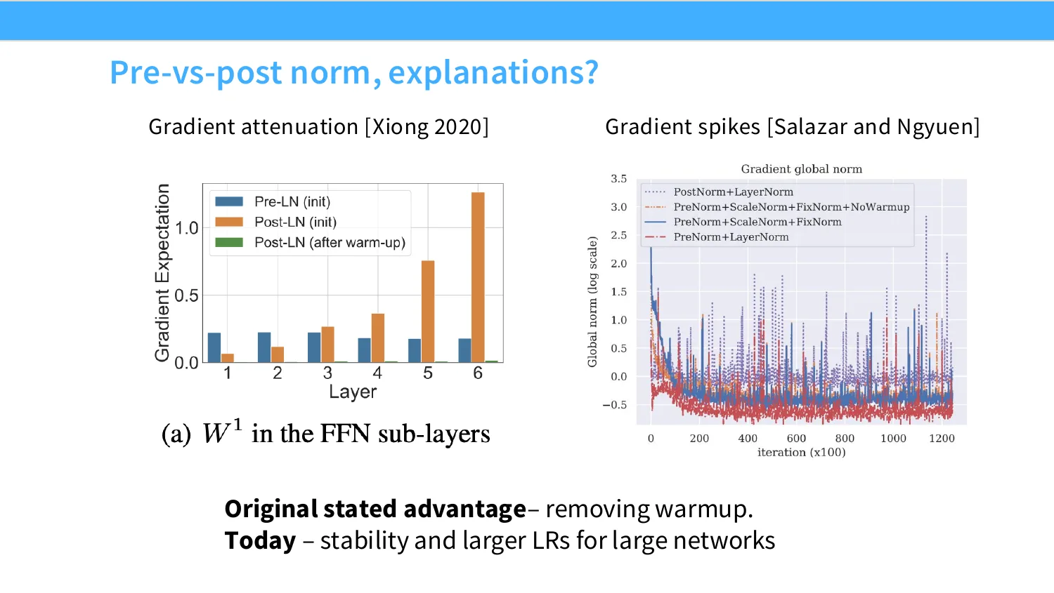
11:25 That makes gradient propagation very simple, which improves both stability and signal propagation. And that's sort of what people realized very, very quickly, that if you do something like pre-norm in blue, at initialization, sort of the gradient sizes kind of remains the same, right? Because you have this nice straight through propagation in the backward pass. On the other hand, if you have post-layer norm, you have these kind of complicated effects that happen because you're layer norming each time you're going through a transformer block. And that's going to change the norm of your gradients as you go backwards through. So you can kind of see, you know, from the principle of keep your residual stream clean, that pre-norm makes a lot of sense. People also realized through experimentation that this also improved stability in general, that the sizes and frequencies of gradient spikes were improved under pre-norm compared to post-norm. And, you know, this is a figure from Salazar and Yuan, who were one of the first ones, I think, to study this phenomenon carefully. And I think this is the reason why it stuck around, right? Stability and the ability to go deep are both very, very important for modern large language models. #

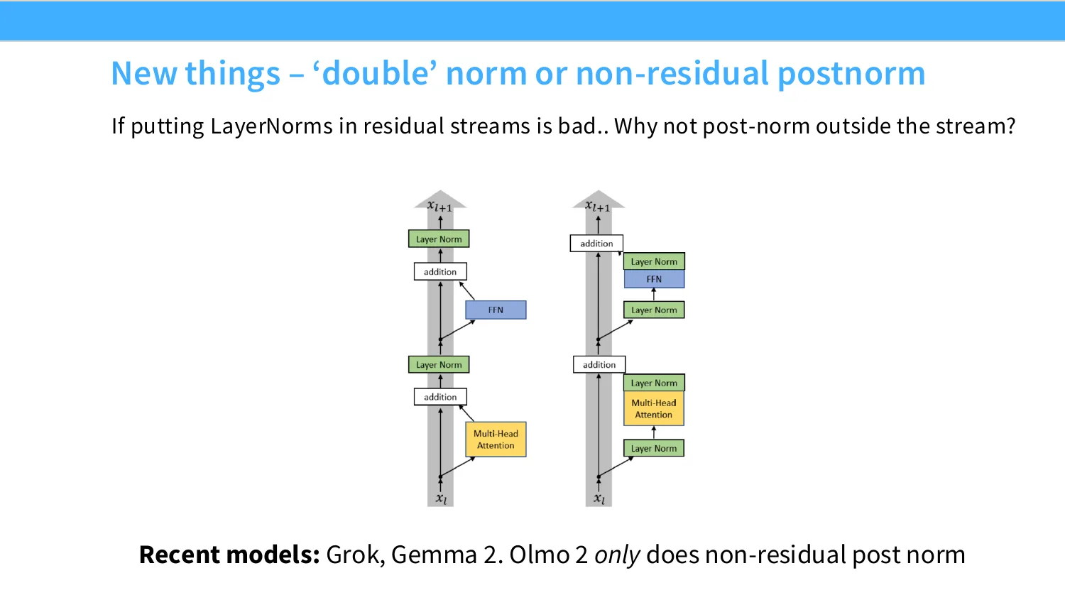
12:37 And so this idea of moving your layer norm outside of the residual stream is one that basically everyone has adopted. So now, you know, if putting layer norms in residual streams is bad, why does layer norm have to be at the start? Of course, we have pre-norm, which is, you know, before our computation, but we could have it after our computation as well, right? That's equally good, at least under that logic. And that's exactly right. Many recent models, like Grom, or Gemma 2, or Olmo 2, have this structure where they've moved the layer norm after the computation. So it's a post-norm of a kind, but it's outside the residual stream. Other models still actually just put layer norms everywhere. They put a layer norm here, they put a layer norm after. #

13:23 I'll get to this later as we talk about stability, but one of the other lessons that seems to have held up very well is if you have stability issues, you can kind of sprinkle in layer norms everywhere, and that will generally improve stability. It's almost very strange to be saying this, because it's so ridiculous. And yet, that statement has actually been proven right. Every time, you know, people have encountered stability issues, they say, oh, but what if we just throw a layer norm into attention? Turns out that works too. We'll get to that later. So, okay, that's post-norm, or double norm in this case, where you have two layer norms here. Okay, the other thing that you can do is in the original transformer, you have the layer norm, which is this operation right here. So you have your activations x, you're going to mean subtract, divide the variance, and then scale it back up, right? And this works just fine, right? It's not like this is wrong. #

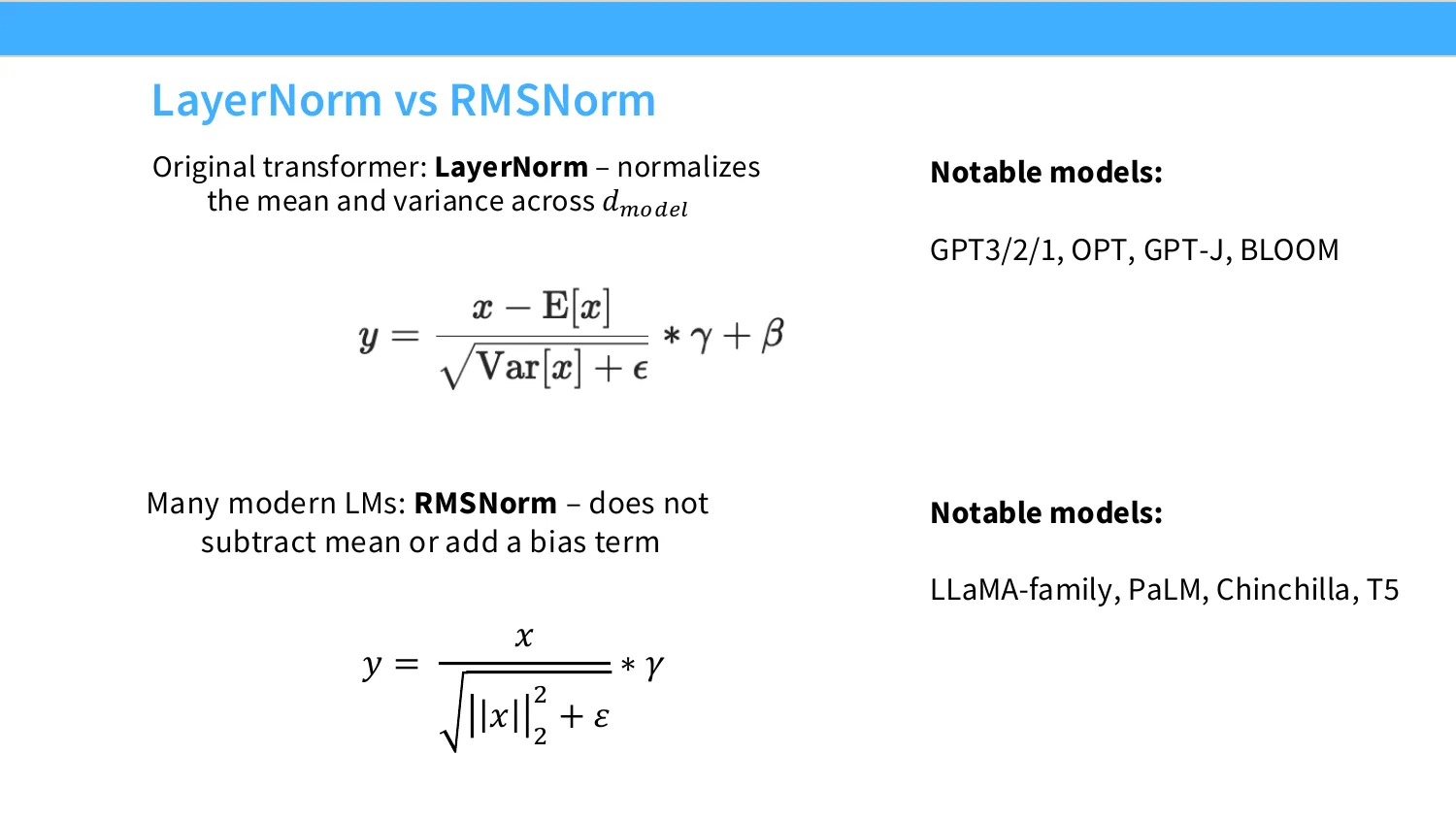
14:11 And many models have successfully trained on this scheme. But basically, most or all modern models, I think, use our mess norm, which doesn't subtract the mean or add a bias term, right? So it's just a scaling down and scaling back up, right? So you can see this in the equation here. And really, layer norm is more expressive than RMS norm. So there's really representationally no reason why you have to use RMS norm. But RMS norm is nice because in practice, there's really no expressiveness lost. RMS norm models just as well as layer norm. But more importantly, it is faster, right? This is #

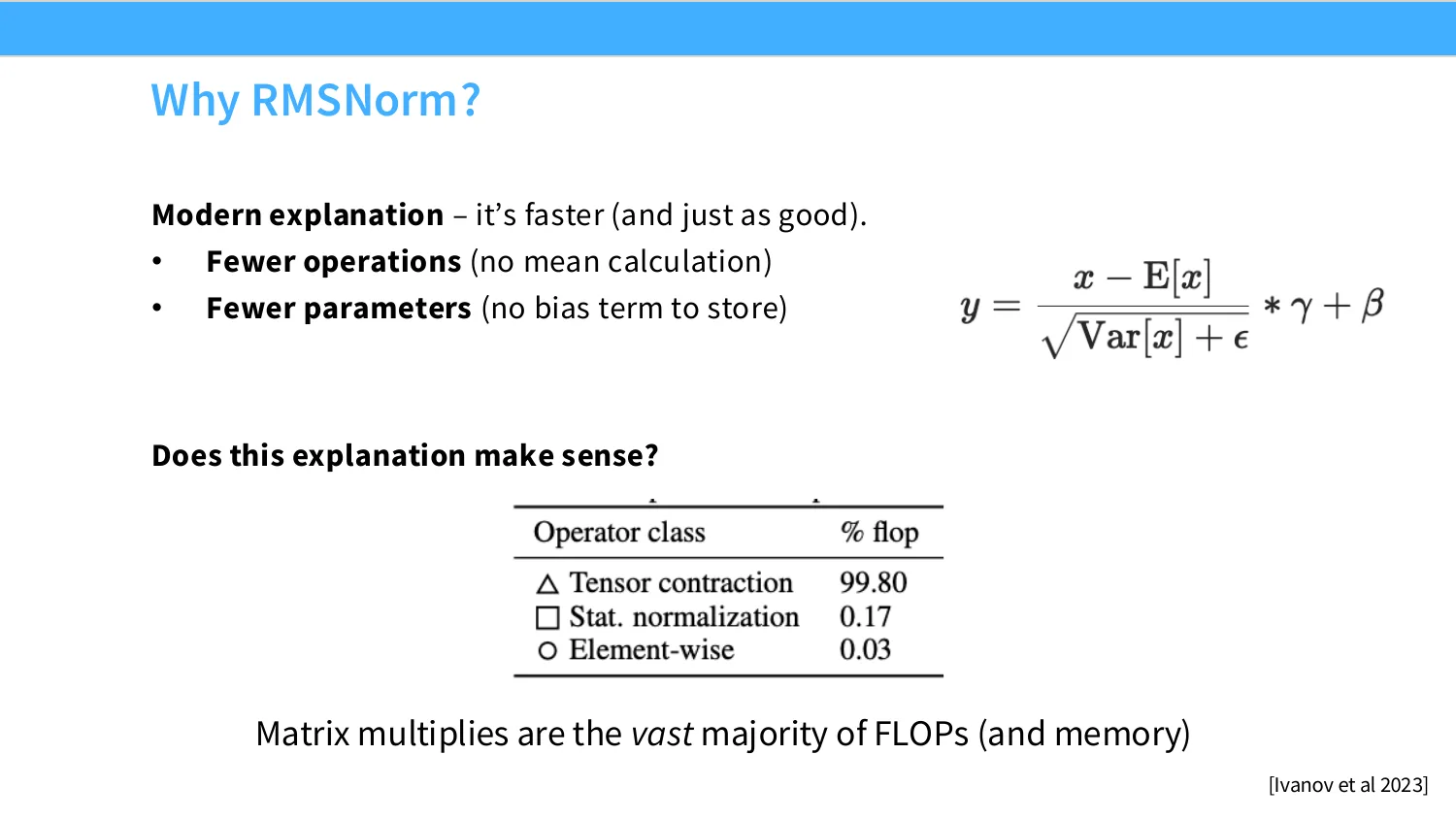
14:50 the part where kind of the systems and sort of architecture co-design starts to come in. Percy mentioned, you know, in the previous lecture, this idea of arithmetic intensity, right? We want to keep our GPUs hot by doing, you know, matrix multiplies and other very intense computations. We do not want to be wasting our GPUs by having them move little tiny bits of memory back and forth, right? That's a very inefficient use of our, you know, operations that are small and involve memory movement, but don't give us much expressive power, right? So by that view, what we really want to be doing here is, you know, if the mean subtraction and addition isn't really doing much for us, just get rid of it, right? You might think, okay, why does this matter? We're just optimizing this teeny tiny operation that accounts for, you know, in this case, something like 0.17% of the total floating point operations of our system. But, you know, as Percy mentioned, it's not really #

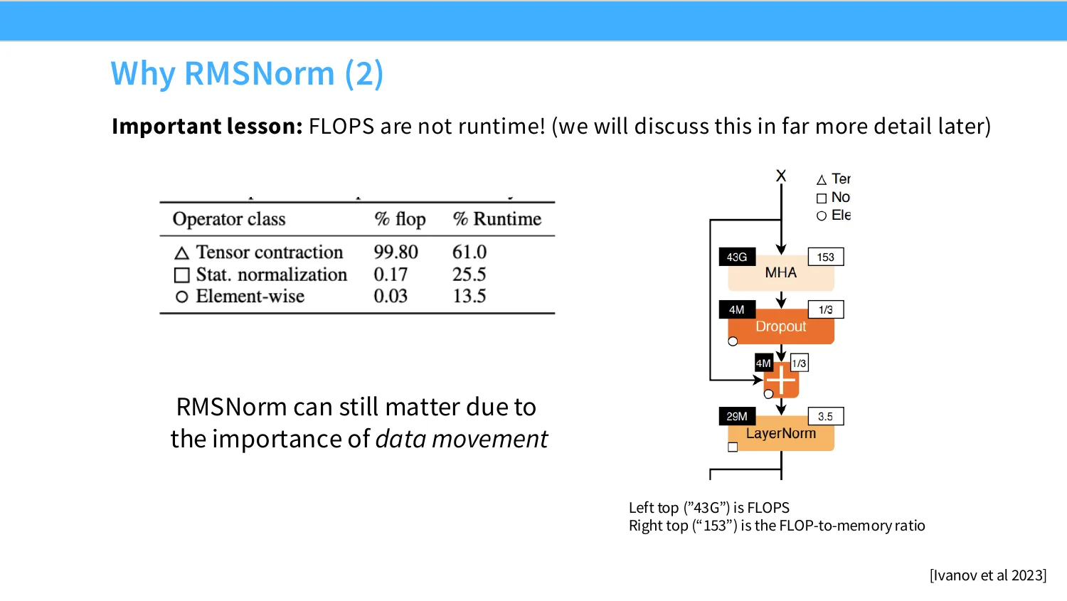
15:52 about the flops, right? The flops are the floating point operations we do, that's sort of multiplying matrices, but that's not runtime, right? Runtime is a much more complicated object, and, you know, statistical normalizations, things like layer norms, even though they're only 0.17% of the flops, depending on your workload and depending on the setup, can be up to 25% of the runtime, right? That's kind of crazy. On tiny models, this can be really, really big, because you're still having to move all these parameters back and forth from fast to slow memory and vice versa when you're doing these operations. So data movement is really, really important, and RMS norm can still matter a lot because of this, right? So you can see kind of the difference here. The arithmetic intensity is in white, and then you can kind of see the flops involved in black, and you see that layer norm has a very low arithmetic intensity, which is the operation we try to want to remove as much as possible. Yeah, question over there. #

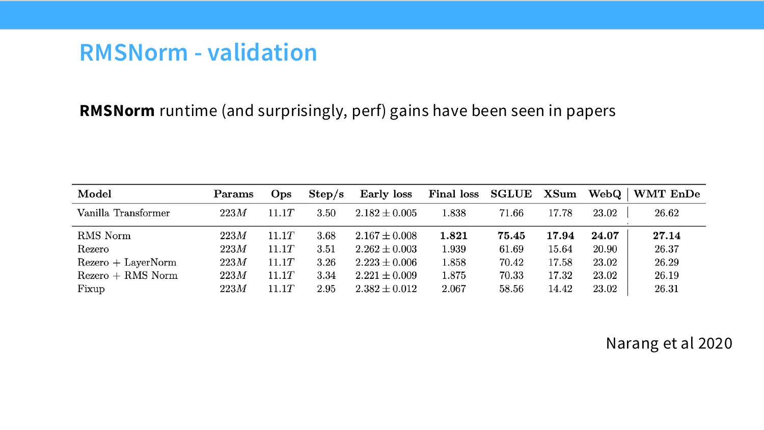
16:54 So for something like tensor contraction, which is in this case matrix multiplies, the majority of the workload is, you know, multiplying, whereas for stat normalization, the majority of the workload is memory movement, and memory movement is quite slow. So imagine the case where like moving something is like almost all of the compute, then you're still paying quite a bit here, right? Because activations can be quite large. Yeah, I think the percent runtime in this case is quite extreme. This is like in the, you know, tiny models with like matrices that don't really generally make sense in modern workloads, but this is, you know, giving you a sense of why this is a free optimization. And you do see this, right? This is another paper in which people were evaluating different architecture intervention. They're wrong at all in 2020. I think this was a Google paper, and they show, you know, for a teeny tiny transformer of 200 million parameters, you get more steps per second. That's the third column over here when you switch to RMS norm. And in fact, you actually get #

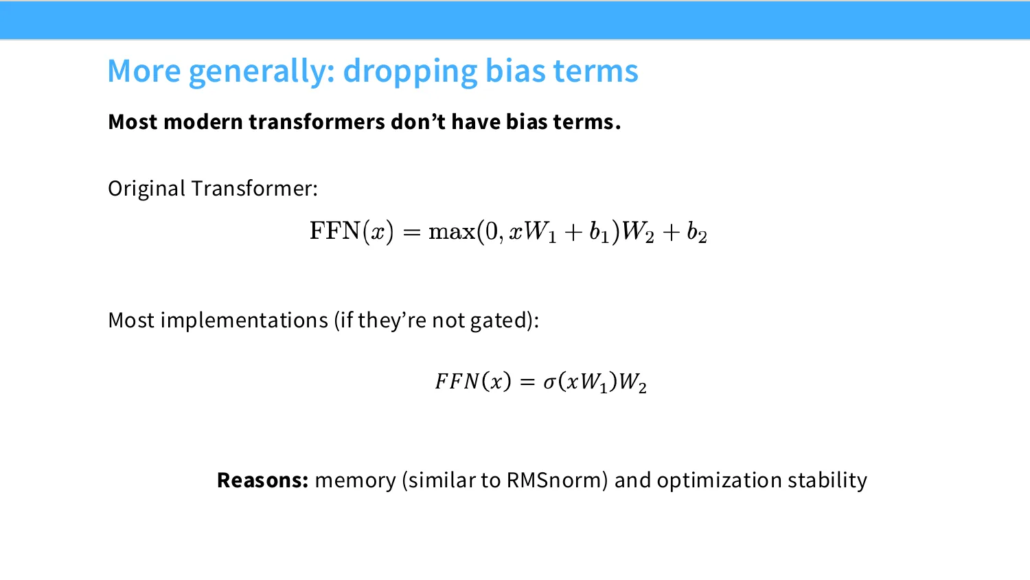
17:49 better performance, which I don't think is something that you're guaranteed, but it's a nice bonus regardless, right? So you get a free systems win by just moving to RMS norm. And so basically everyone has decided to move over to this now. And in general, there's a more general version of this. There's no guarantee to any of the things I'm saying, but bias terms in transformers and neural networks are generally not that useful. So in the original transformer, the linear terms all have biases, but most implementations actually just drop the biases entirely, right? Once again, this is another example of something that's not very arithmetically intense, but fairly memory intensive, relatively speaking. And so you might as well just drop these, right, and get the free systems win. There's also some cases, I'll just mention this offhand, where the bias terms can also induce stability issues. So they're useful in other ways, but really I think the primary reason these are #

18:44 dropped is just to simplify things from the system's perspective. Cool. #

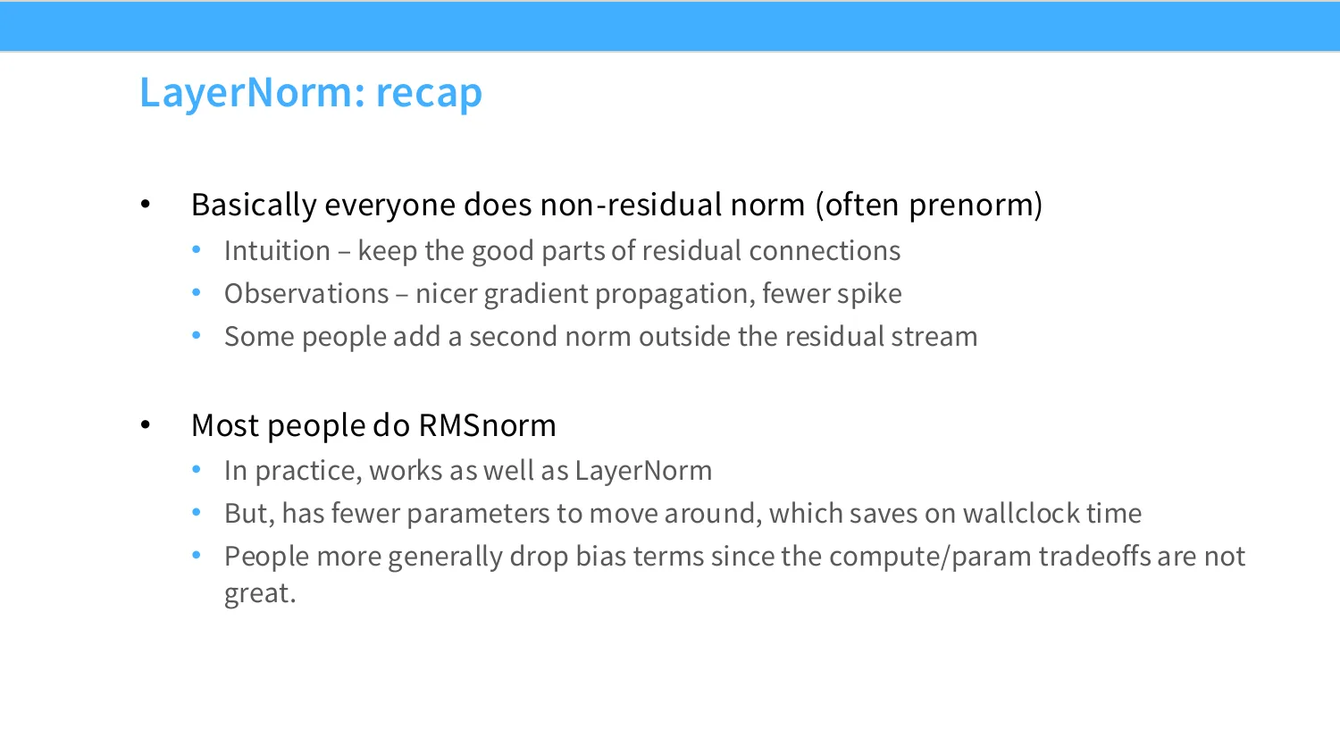
18:51 Okay, so I think layer norms, the story is pretty easy. It's easy in the sense that what people do is fairly standardized. Our understanding, not at like a deep theoretical level, but our understanding of like what layer norm does is fairly good, right? Everyone moves the layer norm outside the residual stream, often pre-norm, but I think this might partially be because LAMA2 did that. And we roughly have a sense of how to use layer norm to control things like gradient spikes and keep signal propagation nice. Related to that, we also now basically always use RMS norm, and you hopefully understand the general principles here of basically just dropping bias terms. And that allows us to keep our system more arithmetically intense while keeping the expressive power the same. I think the unsatisfying thing about a lot of architectures is that you can't really reason about this beforehand, right? Like we don't know beforehand that dropping the bias terms is okay, but from a lot of experimentation and now collectively acquired knowledge, we roughly know that dropping the bias terms on both the linear and RMS norm is okay for typical language modeling #

04 激活函数与门控 FFN（*GLU）

20:01 workloads, right? This is the kind of statement that we can make on the basis of what we do when we look at a variety of different models. Okay, any questions for layer norm stuff? #

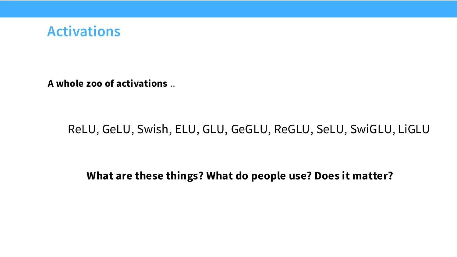
20:13 Good. Okay, so now I'm going to talk about activations. And there's a whole zoo of activations. There's just a lot, right? Like relu, gelu, swish, elu, geglue, selu, swiglu, liglu. And what are these things? I think at one point of my more stats ML training, I thought to myself, I will never learn these things. I will make it a point of pride to never know what a swiglu is. But now it's actually very important for us to actually like have a general sense of what these objects are and which parts of these names actually kind of matter for performance, right? #

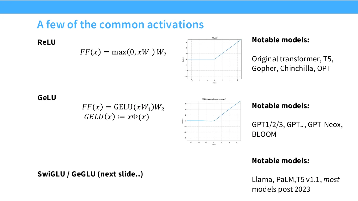
20:51 So you can build and train a language model on just a fairly vanilla activation. Even, you know, I guess chinchilla is probably the best model out of that group. But even if you just want to relu, you know, you can train a reasonably performant language model using just that activation. There's nothing wrong with that, right? And if we move to gelu, which is a gaussian error unit, and really the only difference is this tiny divot at the bottom here, which really, you know, for the most of the activation doesn't change anything, but changes the gradients right near zero, then you can train models like GPT-3, right? That's a perfectly good large language model, not, you know, modern by modern standards, but perfectly fine. But then, you know, we get to the gated linear units like swigloo and geogloo, and these are really where most of the action is. You know, this is very similar to layer norm in that I think almost all credible modern language models use a gated linear unit of some kind. Okay, so what is a gated linear unit? #

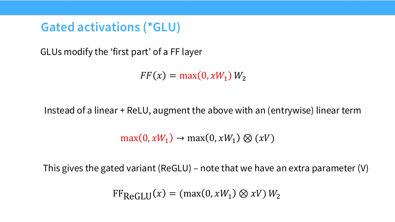
21:52 So these are gated activations. So if we want to look at something like a feed forward layer, we can just look at this first part. This is, you know, a very standard relu feed forward, right? I have my x, I hit it with a w1, you know, I entrywise threshold at zero, and then I hit it with another w2, I get my output, right? Very straightforward relu network. #

22:13 Another thing, I don't say this as my personal experience, but another thing that is often said in architecture design is that gating is often very helpful. So if you apply that very general heuristic, what you might get is to say, okay, well, instead of just having, you know, this entrywise relu, why don't we also have a gate? And the second gate, the second term here, this is just going to multiply the output of my relu entrywise, and I have a second matrix v, okay? Now this is just going to modulate the output of my relu, and then I'm going to do everything else the same, right? So instead of, you know, just having x w1 w2, I have x w1, and I'm going to gate that with x v, this is another activation the same size as this, and then I'm going to, you know, down project it back with w2. Okay, so what is this? Now this is a reglu, this is a, you make these names by adding the first activation, in this case relu, and glu, right? So the relu gated linear unit. And gating has been a, you know, very effective other primitive in architecture design, and it turns out that this is very effective in language modeling as well. So if you take something like a gelu, #

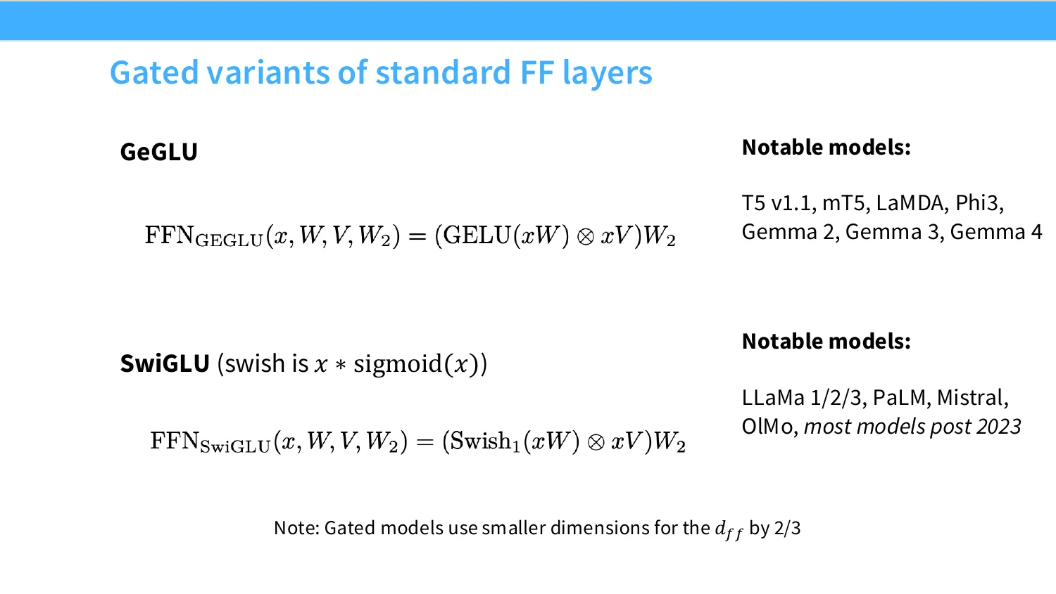
23:27 we've already talked about that, right? That's like the relu, but with a little divot at the bottom here, you will get a geglu. And if you take a swiglu, which is x times a sigmoid, then you will get a swiglu. So this is a swish times, you know, the rest of it. And this really covers a lot of the modern models, right? Generally, the Google folks have used geglu, so like the gamma models, the t5 models are those. And everything that's kind of like a llama descendant uses a swiglu. So palm and the llama descendants are all kind of swiglu models. I would say that swiglu is probably the more dominant one, but honestly amongst the gated units doesn't really matter. Now here's a side note that will #

24:12 be a semi-important piece of trivia later. If you look up here, right, you will notice that there are more parameters for the gated model, right? Because I don't have this parameter of v. And so if you do a little bit of math, right, I now have three matrices instead of two matrices, right? What you should do is you should maybe use a smaller feedforward dimension by a factor of two thirds in order to keep the total parameter count the same, right? So this is roughly the idea of, well, I want to keep the same number of total parameters as my original MLP, but I now want to make it gated. So I'm going to make the feedforward dimension, which is the output dimension of this w, a little bit smaller by two thirds, right? So this is a general rule of thumb that people have followed, but it's not really an iron rule. You know, the original Noam Shazir paper that, you know, proposed this was, had some, you know, very small deltas originally, but they're consistent deltas. #

25:12 And I think to his credit, I think a lot of his papers have these like error bar assessments of like training multiple replicates and checking to see if they're better. And if you look, the GLU variants are almost always consistently better than the non-GLU variants. And this is a parameter matched comparison because Noam Shazir is always doing this two thirds adjustment to make sure that all of the models have the total same total number of parameters. So this is quite nice. It's in some ways a free win. Almost everyone uses a GLU. There have been other sort of more controlled systematic comparisons. This is the same paper I was talking about before, Neurang at all in 2020. Google actually in the 2020s did quite a few nice large scale architecture comparison papers, although with a T5 architecture and not auto-aggressive language model. And they, #

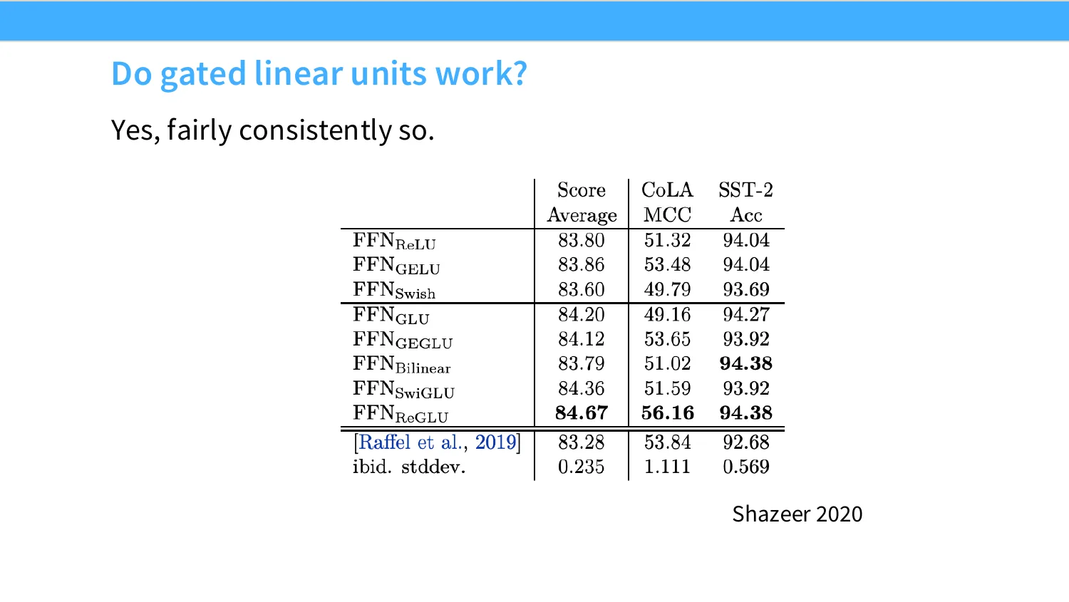
26:07 you know, basically comprehensively compare things like GLUs. And you see once again, if we look at the Swiglu or the Gehglue or the GLUs in general, they do significantly better at loss or the other downstream metrics. Right? Fairly compelling on these papers. Also clear from now a lot of model training runs that Swiglu and GLU are good. Right? So there's a lot of variations in gating, but really the important single axis to know is that gating for these non-linearities is actually quite important. It gives you a nice boost without much of a computational cost. You know, that's not to say that gated linear units are necessary. I mean, GPT-3 was that. I think the #

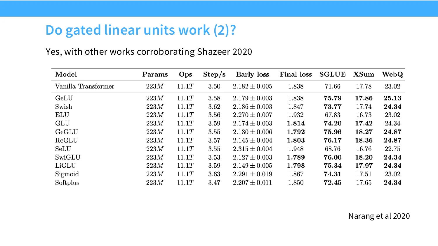
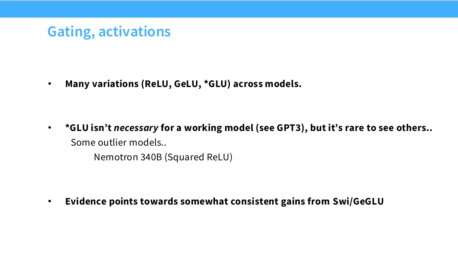
26:50 NemoTron 340b model used the squared ReLU, which is kind of a crazy choice, but that works too. Both of these models are perfectly performant, but it's actually quite rare to see anything that's not trained on a gated linear unit. Right? So evidence is pointing towards consistent gains on using these gating tricks. Okay. So those are, I think, the more consensus choices #

05 串行 vs 并行层

27:14 for things that we can do in architecture. Now, this one, I think, is a really fun idea, but one that I think now the test of time has shown maybe is not quite as good or maybe not as popular of an idea. Normally, we do our transformer blocks serially. Right? We compute our attention, then we compute the MLP. Right? One after the other. If you're very systems-minded, you might say, well, this introduces a bottleneck. Right? I have to wait for the computation of one to do the other. #

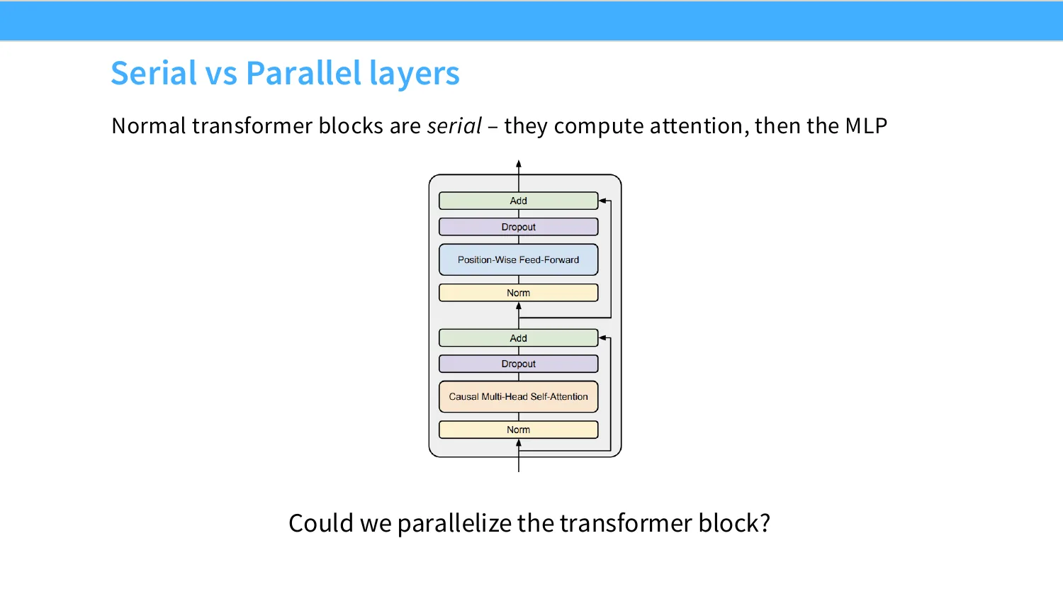
27:41 If they were instead in parallel, I could bring to bear some new and cool systems optimizations, potentially. Right? So you might ask, could we parallelize the transformer block? #

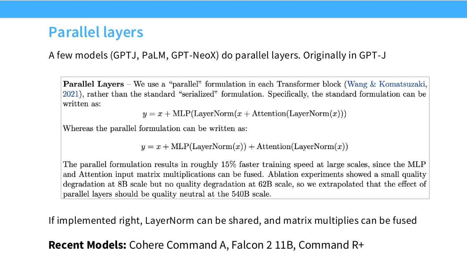
27:52 And this was originally an idea that was in GPT-J, which is the open source attempted replication of GPT-3. And kind of very interestingly, I think GPT-J has been surprisingly influential in sort of propagating a lot of ideas. I mean, Palm as well. Google is actually surprisingly bold with the architectures that they do. But the description in Palm, which you can see in their report, is kind of the following. Instead of nesting this, which is the sequential form at the top, you know, you're just going to add together the output of the MLP and the attention layer and just add both of those back into the residual stream. If you implement this right, you can actually share a lot of the components. Like, you can share the layer norms. You can fuse the matrix multiplies. This allows you to #

28:40 potentially get additional systems optimizations. And I think a lot of the people that have been influenced by Google, so Cohere, you know, was founded from one of the former transformer authors. They do a lot of Google-inspired optimizations. They followed kind of this architecture. But not very many others. This has been an approach that has really fallen out of popularity over the past, I think, two years. I think mainly because optimization of the serial form has gotten sufficiently good that the system's gains from the second one just isn't worth the small hits to representation power that you end up getting going from parallel to serial. Effectively, you can think about it as you've lost half of your depth, right? And that can be a deleterious thing to do to your model. #

29:29 Okay. So in terms of the architecture of things, actually, you know, the fact that this is so short should kind of suggest to you how much the original transformer formulation has somewhat stood the test of time, right? Because the only thing I'm really talking about changing here is, you know, where the norms go, or, you know, whether we have bias terms, or whether we gate the MLPs. But those are actually pretty minor changes compared to all the things that you can do. Now, those of you that are, you know, sort of carefully paying attention might say, but wait, there's a lot of transformer alternatives that change the attention. Yes, you'll have to wait until next lecture, because today I'm just only going to cover sort of core attention-based methods. And next lecture I'll throw in a little bit of state-space model stuff. But as long as you're in this, like, dense attention land, actually the architecture from the original transformer paper is pretty close to what we do. So you see quite a bit of this, right? So just now #

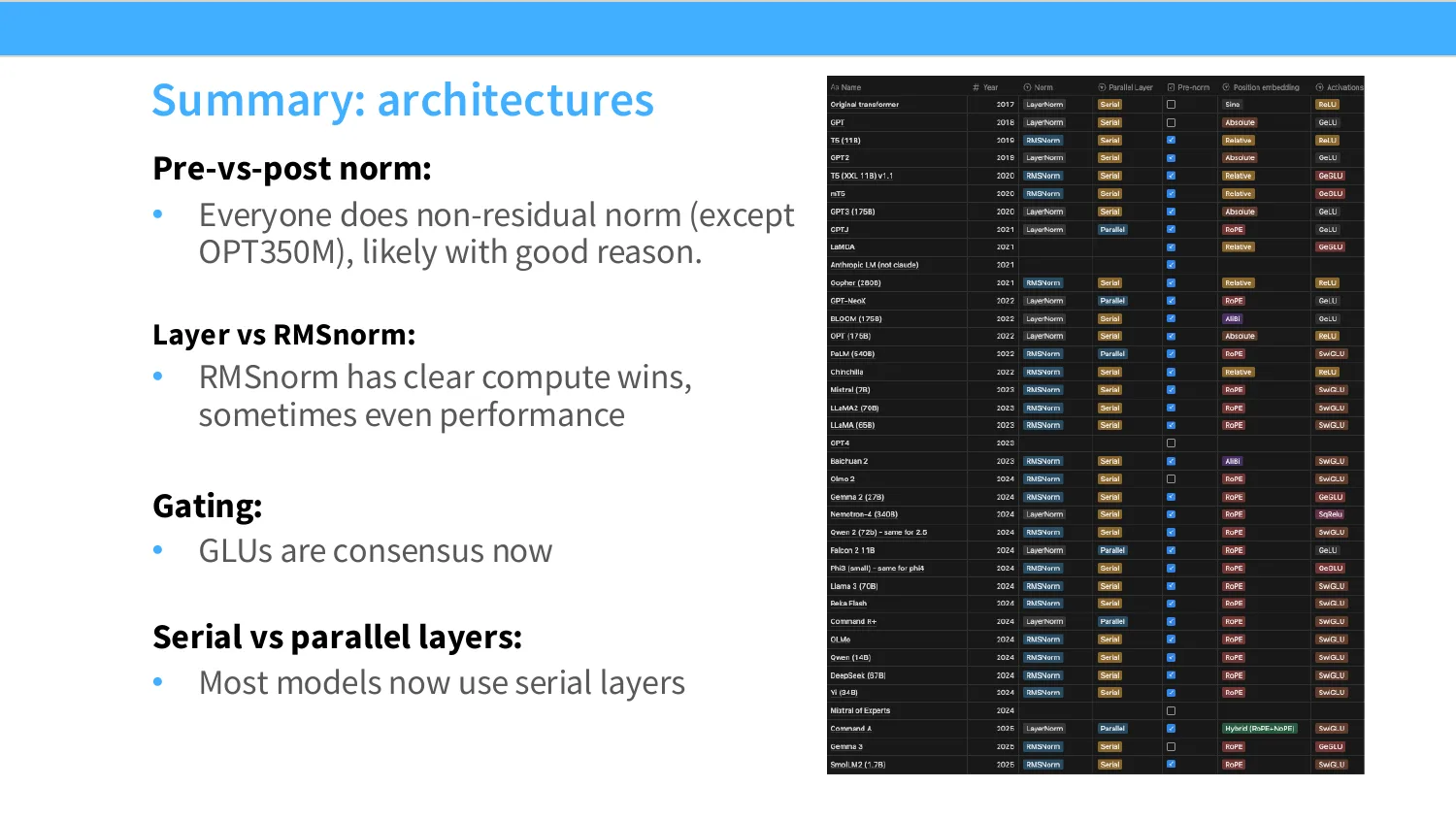
30:26 going back to this, blue here is RMS norm, black is layer norm. You see most of the modern models are sort of RMS norm models. Serial versus parallel layers. The blue one is parallel, the rest is serial. You see mostly serial layers. Pre-norm versus post-norm. Some of these ones that I marked as post-norm are actually pre- and post-norm. And then these ones on the right, these are GLUs almost always, #

06 位置编码与 RoPE 旋转位置嵌入

30:50 with the exception of things like Falcon, which is a gated linear unit. But almost all of these are really gated linear units for modern models. So you can see the trends quite visually from what I'm telling you. Okay, so really the thing that is very different across implementations, and I think a place where a lot of the architecture stuff is still in flux is how you do kind of position dependence and incorporate information from other positions, right? So the core attention component in some sense. So there are lots of different ways that you can encode position into a transformer. And just to remind you, right, this is very, very important because attention is positionally independent, right? They're just inner products, so you can just shuffle them and attention would be the same if you don't have a position embedding. The original transformer had sine and cosine embeddings, kind of like a Fourier transform intuition that if you have sines and cosines, then you can kind of recover position from that no matter what. A number of other sort of large models that, you know, #

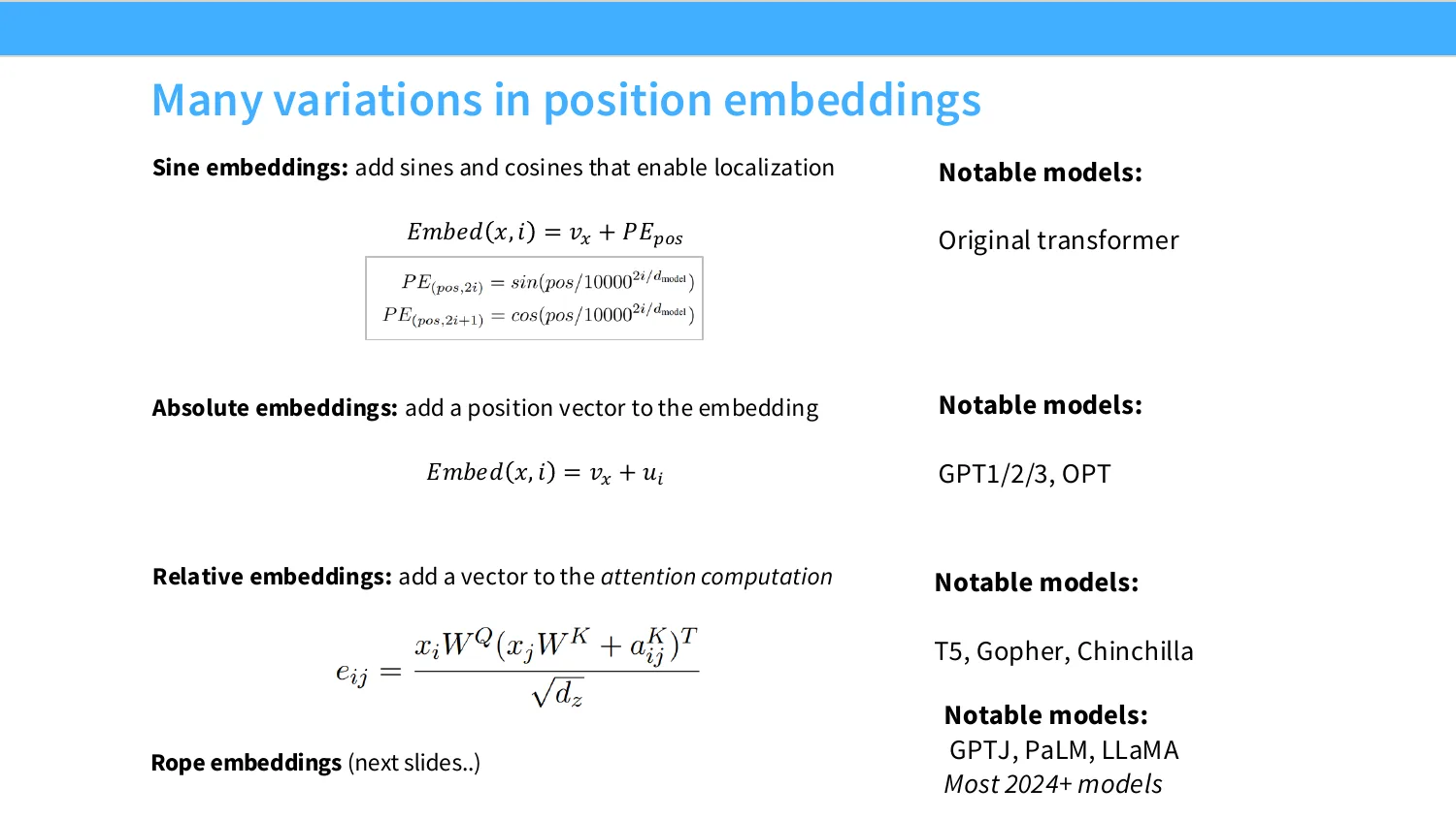
31:52 followed soon after that used absolute embeddings, where each position had its own different embedding. And then several other sort of Google models like to use relative embeddings. And here you're not adding embeddings into the embedding, like word vector embeddings, but instead you're adding a vector to the attention computation itself, right? So if you're three positions off, sort of the attention matrix gets a different offset added to it. And models like T5 and chinchilla use kind of this scheme. #

32:24 The thing that has really become pretty dominant in terms of position embedding is this class of embeddings called rope, which some of you may be familiar with. Most models past 2024 use this type of embedding. And it's kind of remarkable given that rope, you know, in some ways came out of nowhere. Originally, I think this was also a GPTJ innovation from, I think, a sort of not very well known sort of blog post and paper combination from an author in China. But really, it has some really interesting ideas for why you would do something like rope. So rope, you know, is a relative position embedding. And a relative position embedding, let's make an opinionated stance that I should not care about the absolute position of any words. So if, you know, A and apple appear together, even if it appears at the start or at the end, right, in rope embeddings, they should kind of get the same sort of result. And we do know that, you know, or, and we want to sort of represent it in this way, right? So I have #

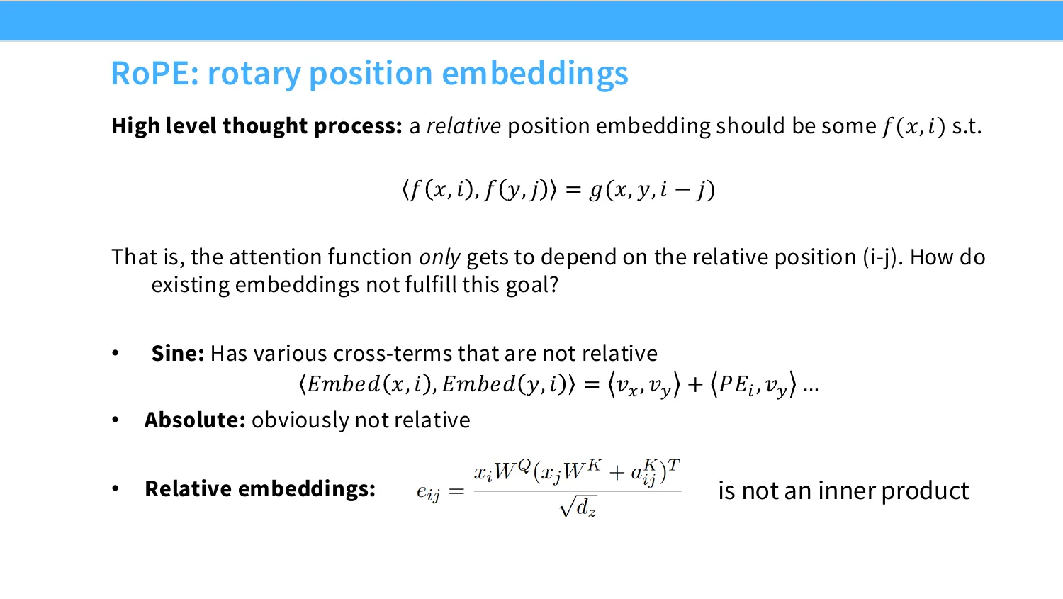
33:31 an embedding F and I have another embedding F, and these are going to take in the identity of the words X and Y and the positions absolute of I and J. And I want this to be equal, if I take the inner product of these embeddings to be equal to a function that only depends on the relative difference. Right? And every existing embedding before it didn't really fulfill this equality. Like, sine is not relative because it has these absolute cross terms that are not relative. Absolute position embeddings just by the name of it is obviously not relative. And then relative embeddings, technically these are relative, but they're not kind of embeddings because they're just adding to the attention matrix, right? So there's no inner product structure that, you know, you can extract out of this guy. So given this, you might ask, is there a nice way that we can truly have this relative embedding? And the idea is very cool. #

34:25 It's really just looking at kind of properties about angles and cosines. So we want our embeddings to be invariant to absolute positions. And we know that inner products of any kind are invariant to arbitrary rotation, right? So the idea is to say, I'm going to take my semantic word vectors, the ones that are independent of any position. So this is my starting point. And then I'm going to rotate each of these vectors, in this case in 2D, based on the position that the words appear. So, you know, just as a simple example, we, let's say we have the sentence, we know that, right? We appears at position zero. So I'm not going to touch that at all, right? I'm just going to keep that where it is. #

35:09 The word know is at position one, so I'm going to rotate it by some angle, right? And that's my one position rotation. Now, what happens if I apply the same idea to the following sequence? Of course we know, right? In this case, we and know are still adjacent. They're right next to each other. But their absolute position has shifted, right? Of course, you know, comes before we know now. In this case, I'm going to rotate the word we by two positions, because it's two index, right? #

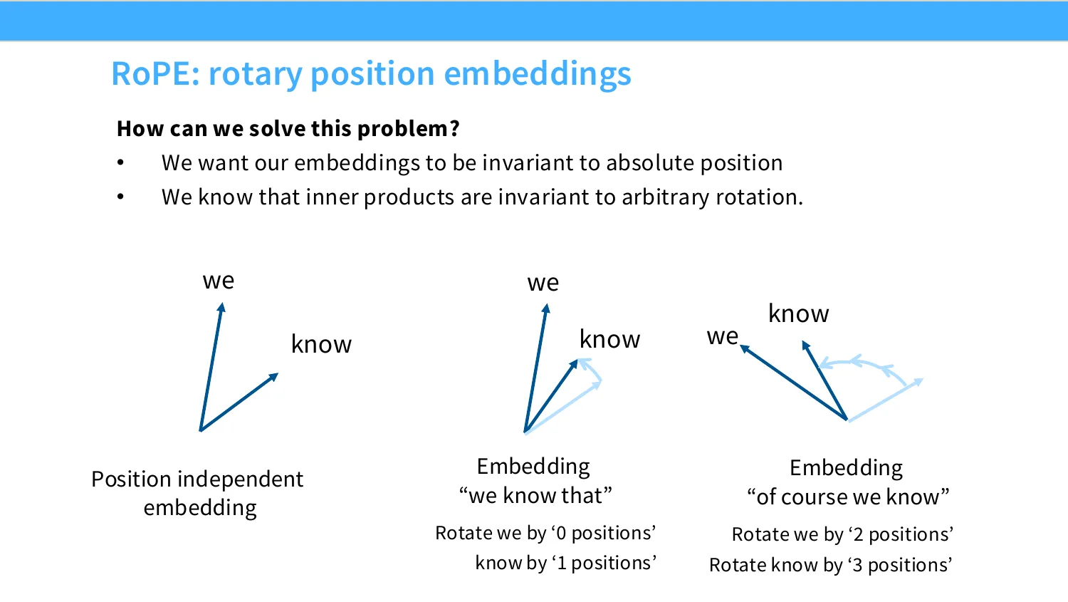
35:37 0, 1, 2. So the word we is in the second position number two, so I rotate by two. I rotate no by three positions, because it's in position number three. And what do you know? The relative angle between these two is still separated by one, right? So this is a very, very simple idea of just using rotations to represent position. And if we do that, then any time we take an inner product, those inner products are going to be invariant of absolute positions. Now you might say, well, in two dimensions, that's pretty easy, because you've only really got one choice. You've got clockwise and counterclockwise. #

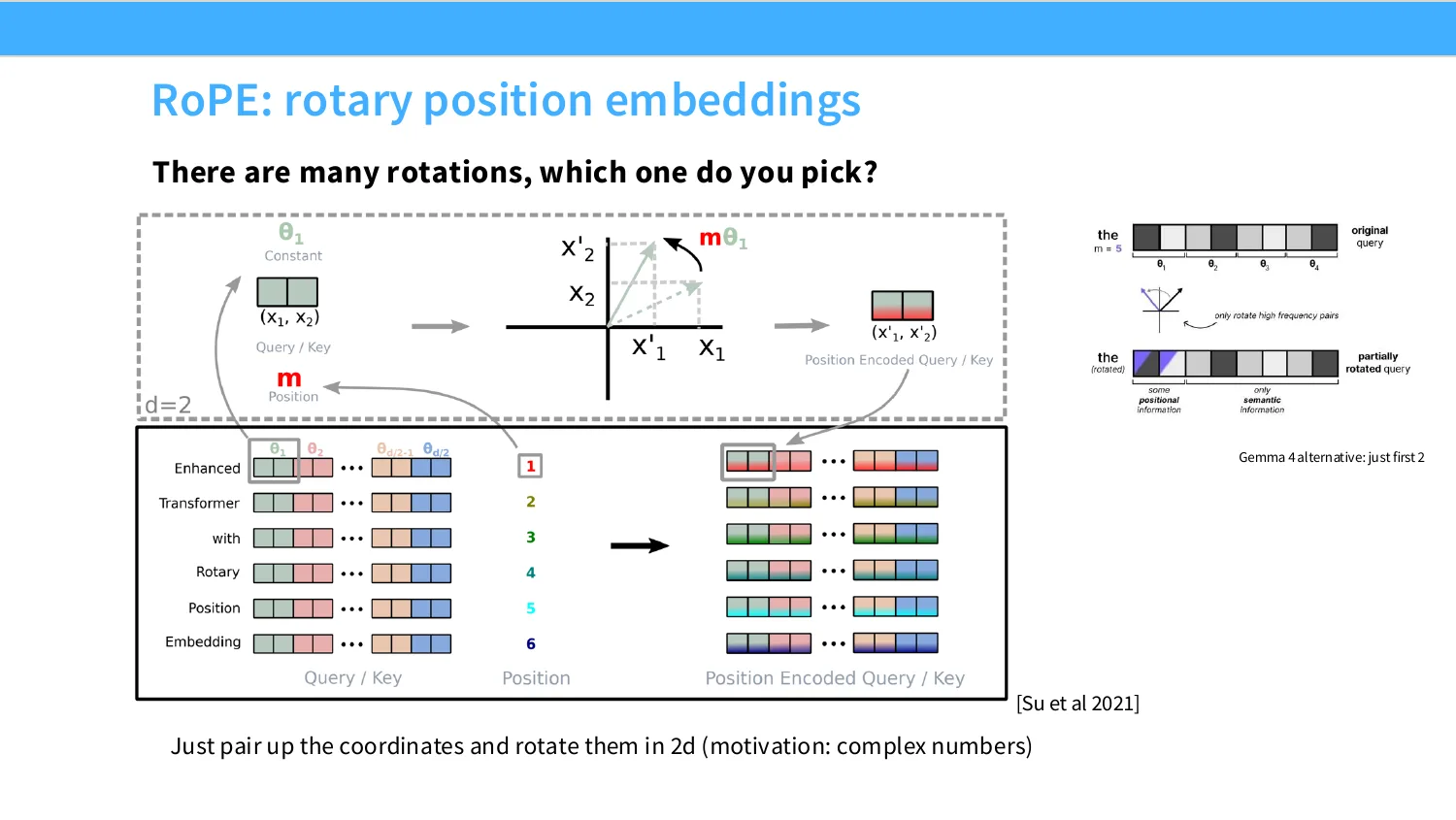
36:13 But in high dimensions, there's an infinite space of ways that you can rotate vectors. So what do you do in d dimensions? Well, you do the simplest possible thing, and it works. The simplest possible thing is to reduce it to the 2D case repeatedly. So you have a d dimensional vector, just cut it up into chunks of two, and each pair of two dimensions gets rotated. And the theta at which these things rotate vary, right? Some of them are very low frequency, so they rotate very slowly, so they can capture long range dependence. Some of them rotate very quickly, so they capture things like, are they neighbors to each other, right? And then at the end, you know, after I've rotated every pair of vectors, I get sort of my final embedding. So this is the, you know, rope approach. The paper, if you read it, #

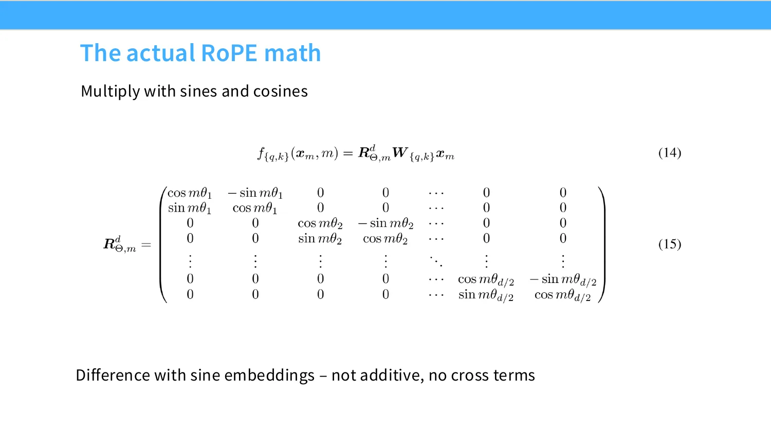
37:00 has a very complex motivation about complex numbers, but really, I think the intuitive way, at least to me, to think about it, is to just, you want to rotate by reducing to the two-dimensional case, and you're just rotating every pair of coordinates. Gamma 4 just came out on Thursday, and they have like another different kind of fun thing that they do, which they call, I think, proportional rope, or p-rope, which is a really strange way to just say that the only thing they rotate is the first two coordinates, but that's another valid thing that you can do as well. So there's a lot of different things that you can do in this space that ends up working. Okay, in practice, what you're going to end up doing is, you know, you can take your vector, and you can make a sparse multiply with sines and cosines, and this is going to be giving you some way of rotating your input vectors x's, right? So x times w times r, this is going to be your final embedding that you get. Okay, and finally, you know, this is a sine and cosine, which looks a little like sine embeddings, but it's really important that I'm multiplying with these sines and cosines rather than using them as embeddings, because that means that there are no cross terms, and this is purely relative, right? There's no absolute position information that you'll get out of inner products. If we really, really wanted to get into low-level details, and you ask, like, how do I actually implement this thing? You know, you're going to have to do that. You have your usual attention stuff, and then what you do is you generate cosine and #

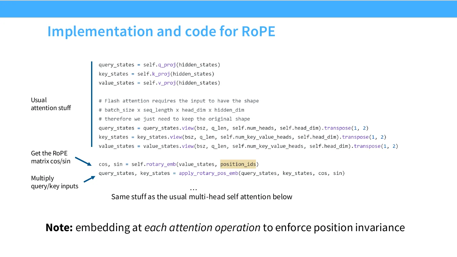
38:26 sine angles based on the position IDs of sort of where your sequence is, and then you're going to apply those cosines and sines onto both your queries and keys for your sort of attention computation, and you can either apply them as a matrix multiply, or you can go through and apply them manually just as a rotation. Right? Fairly straightforward, and you would do this at the attention level rather than at the very bottom to sort of enforce position invariance every time you're doing attention computations. Okay, so that was rope. It is a little bit confusing, but once you understand the geometry of #

07 超参数：FFN 比例、头数与深宽比

38:58 just rotating things, it's actually fairly straightforward. Okay, I'm going to pause here for one moment in case anyone has questions about the various, like, architecture bits. We're going to then talk about even lower-level details about hyperparameters, so yes? #

39:16 Do you know about any papers that do a higher dimensional rotation? Higher dimensional rotations? That's a good question. I don't think so. By a higher dimensional rotation, like any, you know, 2D rotation in the space would just be kind of a variant of this. You could certainly do, like, any one manifold that, like, is a closed loop. I have not seen that. Yes? One, I can ask a question. What do you think is the best way to distill this kind of model? #

39:42 So, papers and vector reports? It's a good question. #

39:49 I don't know if there's a way beyond some combination of, like, looking broadly enough to get a pattern, which is the procedure I'm trying to do in this lecture here. And then the other one is to try it yourself, even a much smaller scale, to form an intuition and, like, a theory for how these things come together. I think those two are really the right ways. I think reading any single paper in isolation is very, very difficult, especially now, because no single paper seems to give any full detail for a lot of language models these days. #

40:17 Oh, lots of questions now. Okay, good. We'll go ahead. So, I have a question on the parallel layers and the serial layers. I understand the modern models are thinking of the resource of anything, so they will use the parallel layers. Yeah, but there's a difference between the accuracy for these two patterns, right? I want to know, what's the, what's the, what's the, what's the, what's the, what's the, what's the, what's the big enough to, is it small enough to allow the current model trailers to hit it all at, or is it any? Yeah, I think, you know, the, that's actually really mixed. So if you read the original palm paper, I think they're like very confident about the use of parallel layers, like no performance drop, 15% systems utilization improvement. So if you read just that, you'll kind of say like, oh, #

41:04 it's just as good. But I think a lot of the, the later Google models have stopped using this, which you can take on as an implicit signal that actually there might be some losses. And once again, this one is a little bit hard to, to get precise numbers on, because no one's done the ablations, as far as I know, on parallel versus serial. Controlled nice ablations at least. Yeah. #

41:27 So, what's the difference between like, the diesel central, the diesel central, the diesel central, the diesel central. #

41:34 Yeah, yeah, I mean, this difference is really just like, which of the coordinates you rotate. Like you don't rotate most of them, because a lot of the, I mean, the argument originally, I think, is that the low frequency parts just aren't rotating very much. And so you can drop them if you're really strapped for, you know, sort of extra space. And this is really an optimization for teeny tiny models, where like, you don't have very much like, hidden dimensions to have activations for. Yeah. For the relative embeddings, not having an inner product, is that because it only applies to keys basically? I was trying to understand. Yeah, so they apply both to the keys and values, which is kind of why, you know, you get this like relative effect from where you are. You want to not have cross terms, right? So if you look at the sine and cosine embeddings, then you'll not only get sort of the, #

42:27 you know, the original vectors. You'll kind of get these weird cross terms between the position embeddings and the word embedding themselves, and so on and so forth. And then you can kind of back out what the absolute position is. So even sine and cosine embeddings are not like pure relative position embeddings. You know, you have to accept the premise that, you know, the relative embedding is what you want. But once you do, kind of you end up at the rope solution somewhat naturally. #

42:57 Yeah. Yeah. #

43:01 So the issue with this is that it just can't be factorized as a product. That's more of an aesthetic problem, right? Like if your constraints are, I need it to be relative and I need it to factorize as f of xi and f of yj, then this is not a solution in that class. To be fair, there's a lot of embeddings that work this way, that do work, like alibi and other kinds of like approaches, like do do this kind of inject into the attention matrix, and they do reasonably well. It's not necessarily the one that's become the dominant approach is what I can say. #

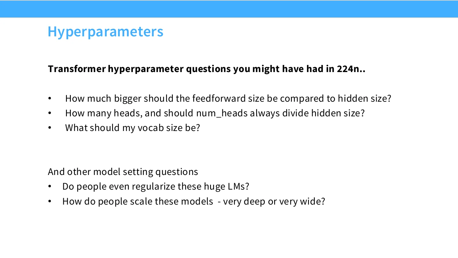
43:36 Cool. Okay. Great. Okay. Now I'll talk about hyperparameters. And I think hyperparameters are really something that you start to engage with once you like actually have to train a model, right? When your knowledge about language models are abstract, you don't have to care about any of these. But once you have to instantiate it, you start to ask questions like, well, how big should the feedforward size be? How many heads should I have? What should my vocab size be? #

44:03 Right? And you might also have questions of like, what should my weight decay or dropout be? Like, do I even need to regularize? I have a lot of tokens, right? So do I need regularization? And do I need very deep models or very wide models? Like, what are the right kinds of things to do here, right? In all of these, if you start out with no knowledge, it's actually very daunting because you have to search this like very big high dimensional space. But the space of things that people try is actually pretty small. And from that, maybe you can start to think about, you know, smarter search #

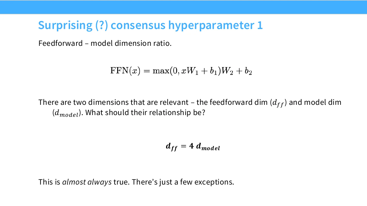
44:33 processes of like, where you want to vary things. One of the things that's a really consensus hyper parameter is this idea of the ratio between the feedforward size, which is kind of the output of your first matrix multiply in an MLP, and the model dimension, right? So this is really the ratio of the two dimensions of your W1 and as well your W2 matrix. This seems like a thing that's very important and controls kind of the richness of your MLPs. So what should it be? Well, for whatever reason, it should maybe be four times your hidden dimension, right? And this is a rule of thumb that works remarkably well. And I will show you some data on like why maybe this is a fine number to choose. There's a few exceptions. And funnily enough, the really extreme exceptions kind of backtrack on that. #

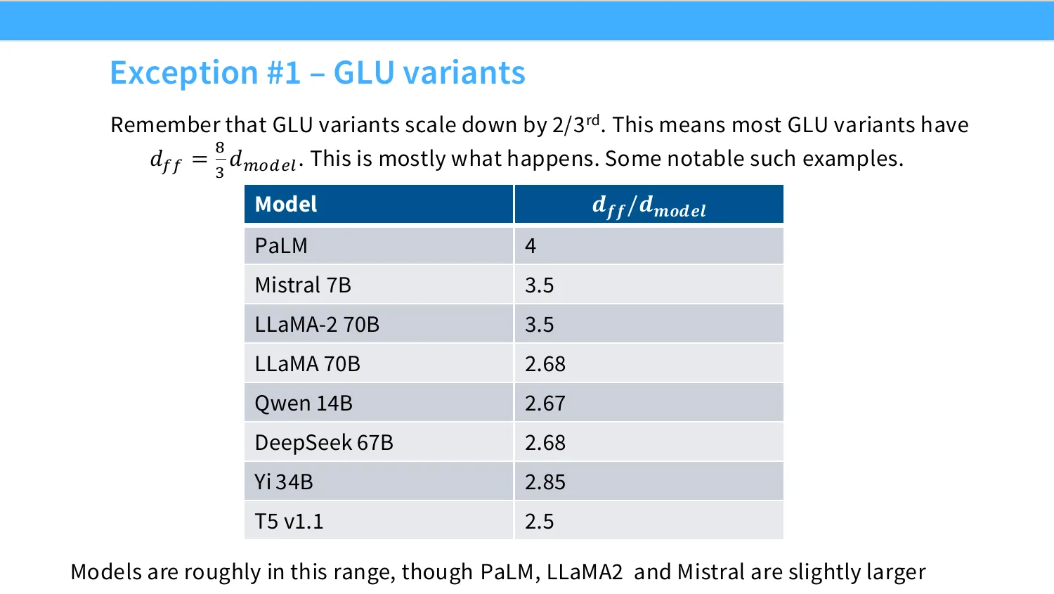
45:26 Okay. Exception number one is variance of the gated linear unit. I already told you about this, so if you were thinking about it, this is probably cached in your head, right? GLUs have more parameters, right, if you keep the same dimensions. So if you want to keep the parameter size of your MLPs the same, well, you need to scale down by two-thirds, right? So most GLU variance, this means that you're going to end up with something like 2.67-ish, right? So everyone that's down here, 2.67 to 2.5, #

45:56 this is roughly applying this like two-thirds correction. And then for whatever reason, the LAMA2 folks decided, well, we actually have very efficient attention heads with like MQA, which I'll talk about later. And because of that, we can multiply this ratio by an arbitrary 1.33, and we'll get roughly 3.5. And so the LAMA people kind of like arbitrarily chose a slightly different ratio, which essentially emphasizes the MLPs a little bit more. But really, if you actually look through all the papers, you'll find either 2.6-ish or 3.5 for GLUs, or 4 if you're doing non-GLU models. Okay. There's another exception which I find to be very funny, #

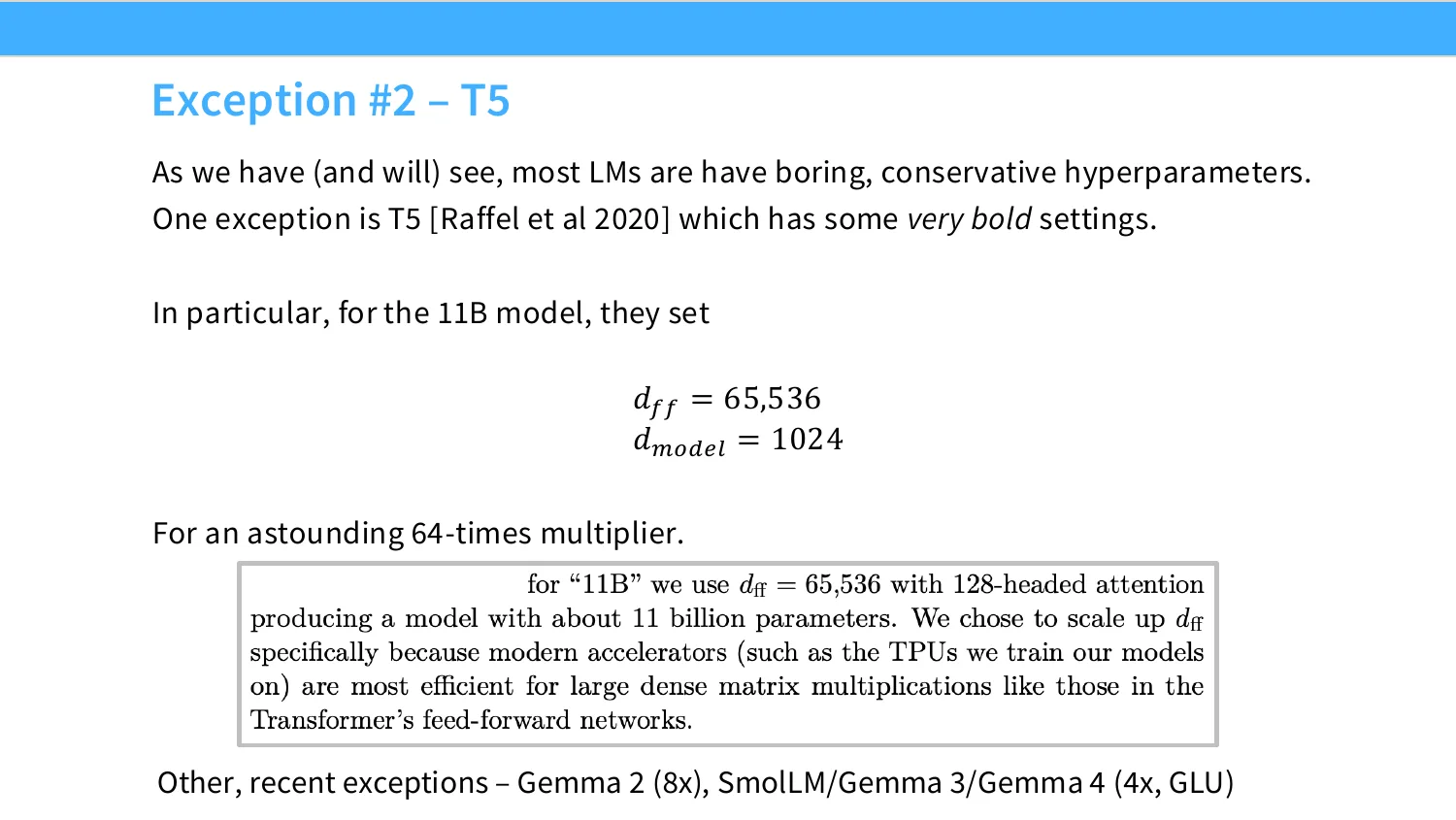
46:44 but also very, very cool, which is, you know, throughout, as you read these like technical reports, you'll find that most people are just very boring in their choice of architectures. They're like, we did LAMA, but we changed one thing. But, you know, folks at Google are very bold sometimes. And T5 is one of my favorite ones, because they have some really bold settings. They decided that instead of following this like 4x rule of thumb, they decided that they want to have a 64x multiplier, which is like way bigger than 4. And they have a reasonable argument for this as well. This is another like systems-based argument, right? They said, well, you know, if the bigger my matrix multiplies, the more efficient I can keep my hardware. So if I make this, you know, multiplier really big, then, you know, my matrix multiplies can potentially be sort of more efficiently utilized, right? And some others like gamma 2 have also tried to really push a little bit higher on this. #

47:44 But really, T5 is an kind of astounding exception at 64. I don't think any other model has really gone that high in the feed forward multiplier. And empirically, if you look at other sort of works that try to do more controlled comparisons of this ratio. I've taken this one from Kaplan in 2020. This is the classic neural scaling loss paper where they do sort of various controlled studies on language models. You'll see, you know, this wasn't the point of the study, right? It was a scaling loss study. But you'll see in one of the panels that they actually have a sort of ablation or a sweep where they change the feed forward ratio and they look at the loss, right? For a very small model here, right? But what they #

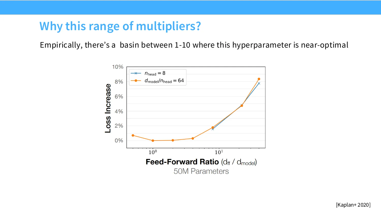
48:27 find in this paper is there's a basin where you start at about one and you end about maybe 10, where this hyperparameter is like pretty good and very, very flat. You lose very little relative to the optimal loss down here, right? And then if you get it really wrong, like you get, you know, above 10 to 100 or something like that, you know, then your loss starts really shooting up quadratically. And so a lot of these choices that range between like 2.6 to 4, they're all kind of falling into this relatively nice basin. So you're fine choosing those numbers, right? Okay, so what can we learn about this hyperparameter? Well, the default choices have worked very well for nearly all modern language models. So you can safely choose that. T5 was a fine model, or the #

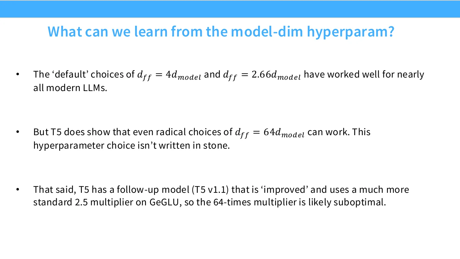
49:11 virgin 1 T5 was a fine model, right? Like it wasn't a bad model. And so even radical choices can technically work, but it's probably going to be compute inefficient. And I think the funniest part of this saga of this kind of the punchline of the T5 saga to me is that they have a follow-up model T5 V1.1 that's like supposed to be the improved version of T5, and they kind of go back to the standard 2.5 multiplier, you know? So there's nothing explicitly stated here, but clearly, you know, when they tried to update T5, they decided that they wanted to go back to a more standard multiplier, which I find to be a little bit funny. Okay, so that's the, you know, feed forward ratio, which now you have like a rough sense of like what the right order of magnitude is. Now let's talk about a different consensus hyperparameter. I always found this to be very strange when sort of teaching 224N and, you know, #

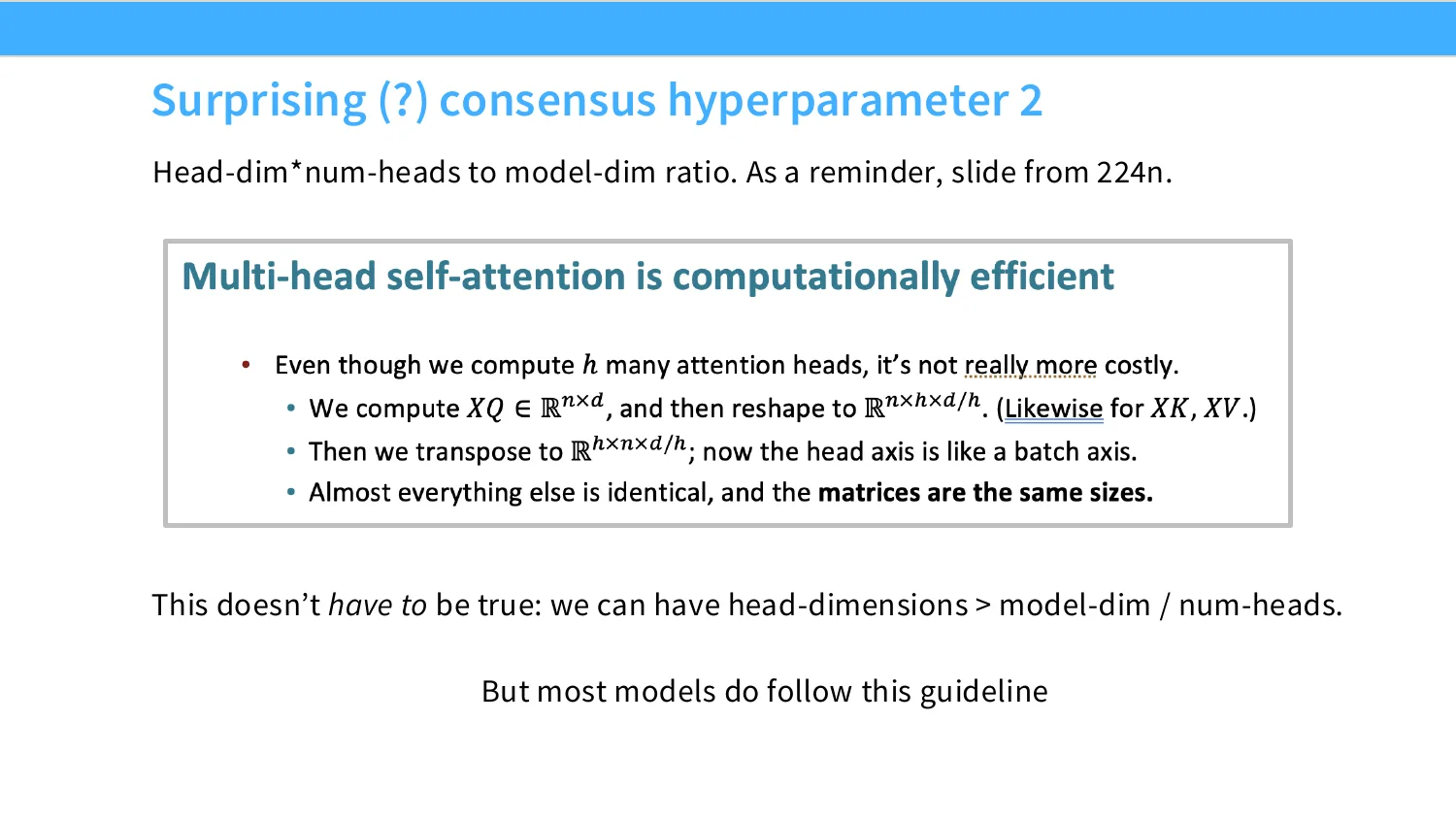
50:02 just sort of teaching students about this, which is if you have a multi-head attention, where you have multiple heads for your attention in your transformer, the canonical thing to do, the thing that almost everyone does, is if you have multiple heads, you make sure that the size of those heads, the head dimension is such that you sort of have the same dimension as a single head transformer, right? So you always make sure that you sort of divide the hidden dimension to basically multiply with H. So in this case, right, you have H, the number of heads, and the dimension of each head is D over H, so you multiply the two and you get D, right? For some reason, this is kind of the rule of thumb. Of course, this doesn't have to be true. We can arbitrarily change the ratios between head dimensions and model dimensions, but most models do follow this guideline, and it turns out to work pretty well. And we can look at a variety of different models, classic and new. I have the latest and greatest coin as well, and you kind of find, yeah, the ratios are roughly around one, a model head. You know, notable exception of T5, and even lambda, which is another Google model. But really, everyone sticks around one, and I think this is kind of an #

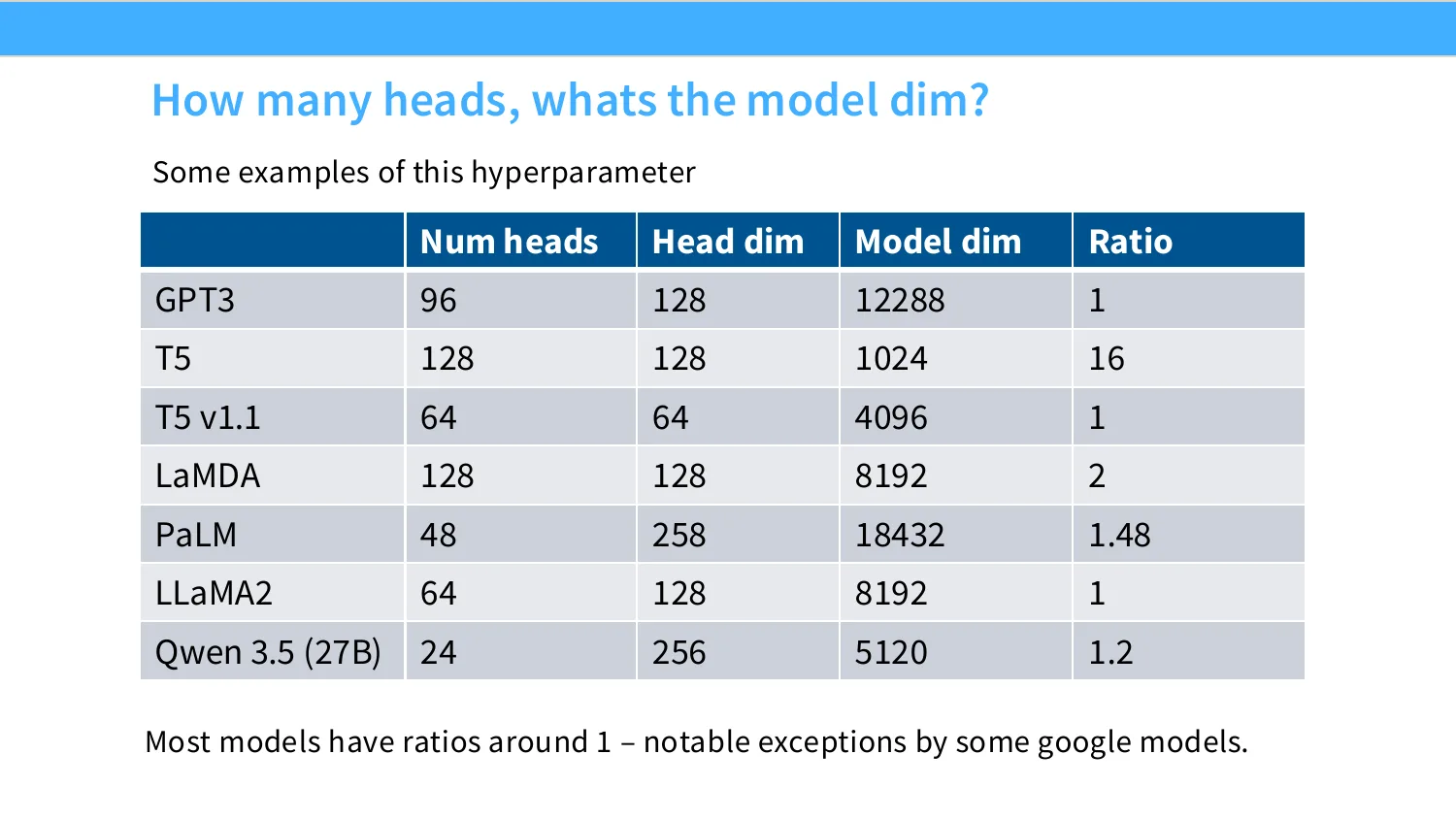
51:11 interesting one. I think the thing about head dimensions that I'll end with here is I think this is yet another kind of forgiving hyperparameter. There's a couple of ablations that people have done. There's, once again, a pretty wide basin around one that you can sort of get away with. OK, but that one's maybe not the most critical hyperparameter. I think maybe one of the most critical and interesting ones, I think conceptually, is this idea of an aspect ratio, right? And sort of to add an extra point here. When you scale models up or down, the way you usually do that is you fix an aspect ratio, like how wide your model is versus how deep it is, and then you make the whole model bigger, right? So the aspect ratio in some sense controls the entire depth to width trade-off as you make models bigger, right? Now, you might wonder how deep should my model be? Like if you've been #

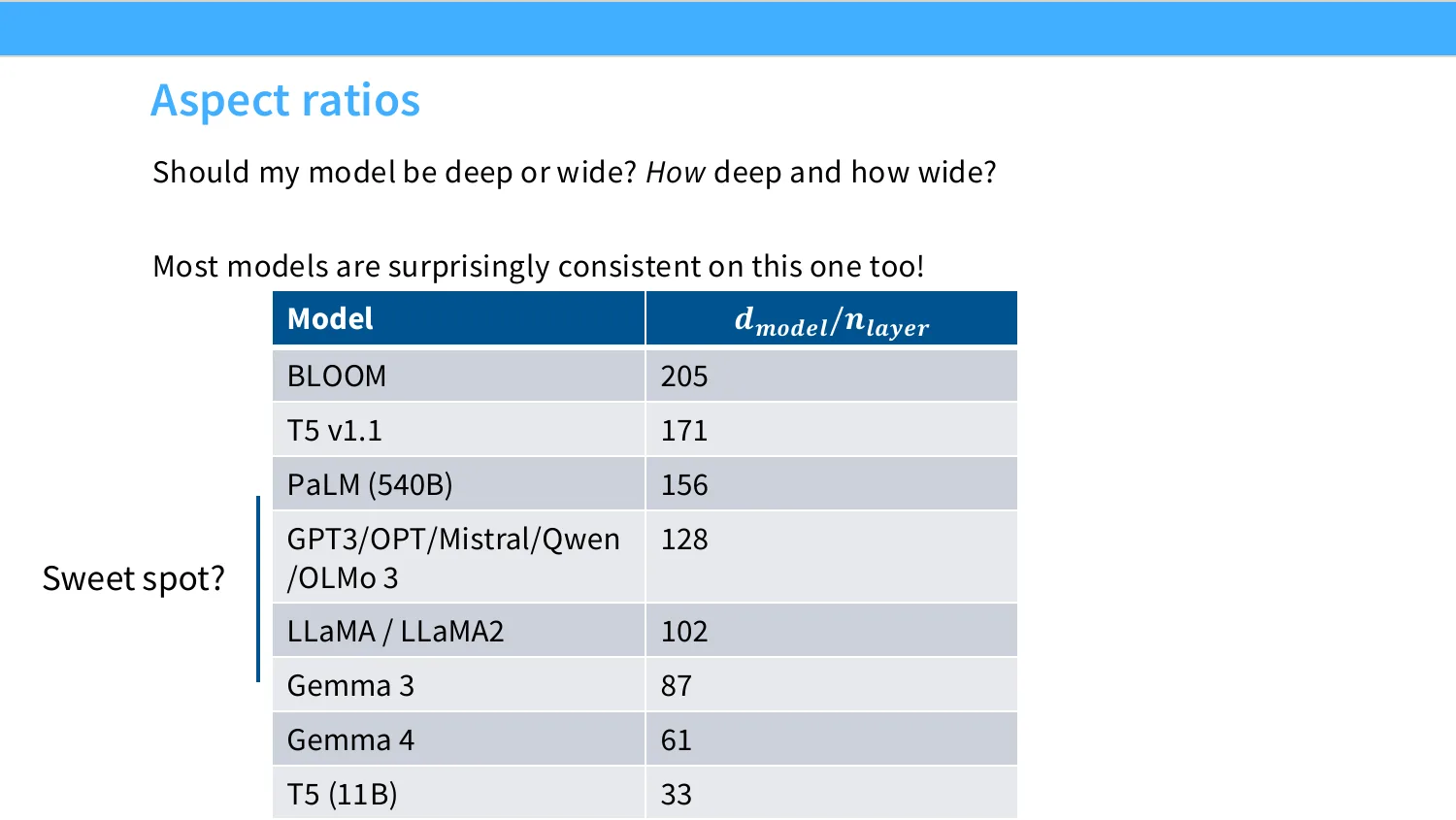
52:00 following all this stuff on like reasoning and so on, you might think I need a really deep model or a shallow model if I want systems utilization. You might think that there's a lot of sort of variation. And there is a lot of variation, much more so than other hyperparameters. But there's actually like a fairly clear sweet spot that most modern models fall into. You don't really see models go like too deep, and you also don't see models go too wide in either direction, right? You see most models have a ratio of about 100 D model over N layers. So about 100 sort of width for every layer that you have. I mean, this is true for like GPT-3 or LAMA or any one of these models. #

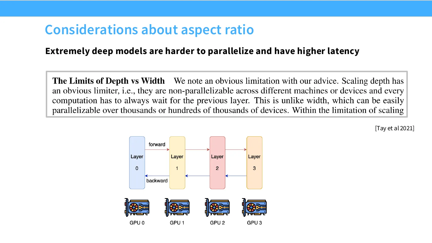
52:44 And really, I think the considerations are partly a trade-off between expressiveness and hardware, right? If you have an extremely, extremely deep model, they get very, very annoying to deal with systems-wise. The deeper your model, like what is the ways that you have for paralyzing them? Well, you might have to cut up your layers. If you cut up your layers, we'll talk about this in the systems lecture. Once you start cutting up your layers depth-wise, you have very serious issues in paralyzation. Pipeline parallel, which is what this is called, is something that like most people really, really do not want to deal with. Whereas width is much easier to paralyze. If you have a really wide model, you can cut that up very easily in your GPUs. Tensor parallel is what it's called. It's much, #

53:26 much simpler to deal with. And so in some sense, there are systems reasons to go wide, and maybe there are expressiveness reasons to go deep, and you end up at roughly 100. #

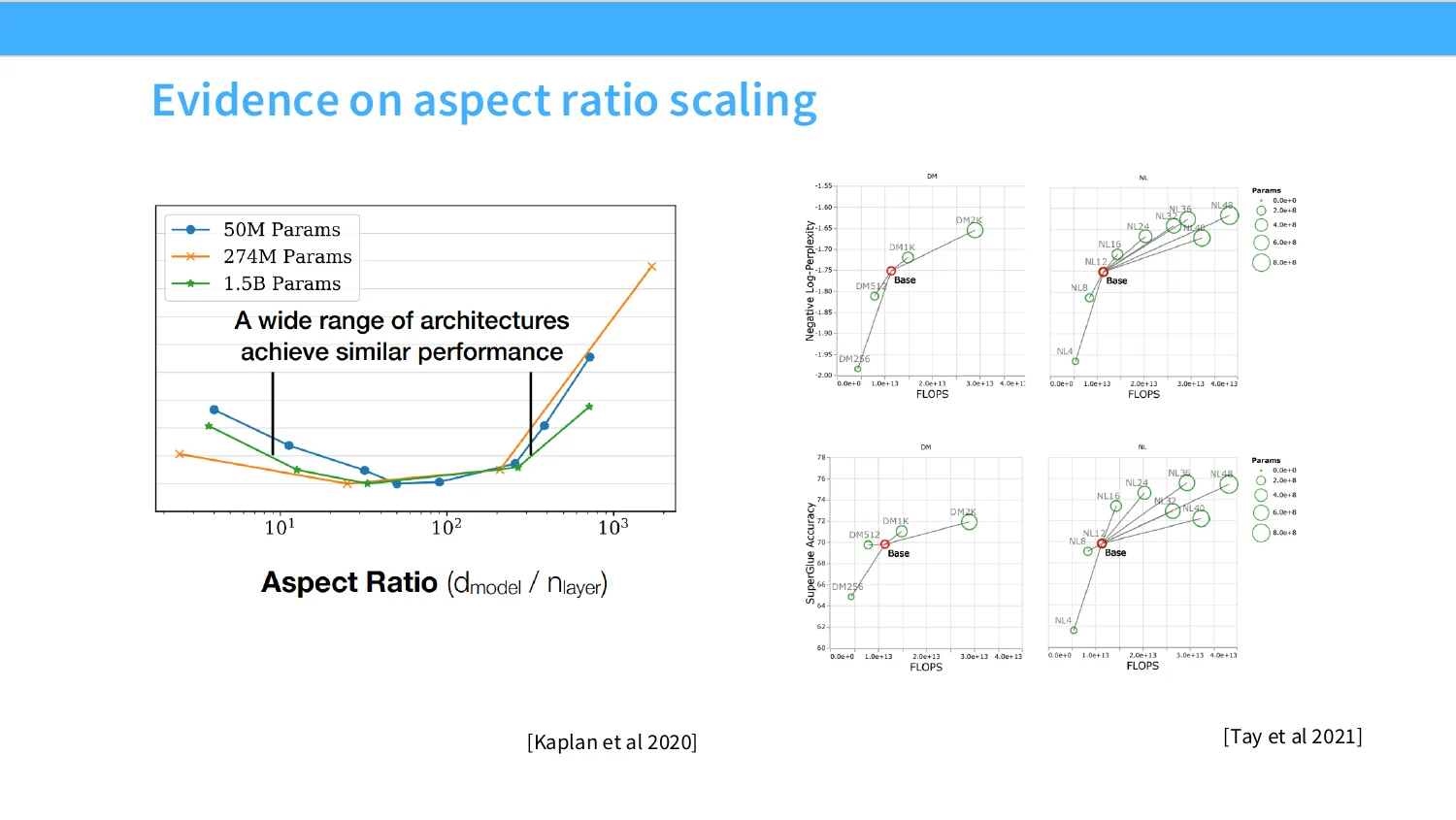
53:39 And I think one of the really interesting things about transformer hyperparameters is there are a lot of hyperparameters that seem quite important, but they're also fairly forgiving. And people have converged roughly on the minimum. This is yet another plot from Kaplan et al., which shows another sweep over hyperparameters for differently sized models. And once again, you see, regardless of kind of the size of your model, roughly speaking, the optimum aspect ratio is fairly similar. And they live at about 100, maybe a little bit less, depending on how you want to do the accounting. But really, anywhere near 100 is a pretty safe bet for aspect ratios. E.K. and others did a number of really interesting sort of like architecture #

54:24 architecture variation experiments, in which their general conclusion on this was that, let's look at the top panel here, you have a lot of different kinds of models that you can have in terms of depth to width tradeoffs. But as you sort of sweep the depth to width tradeoffs, you find that really the only thing that matters in some sense is flops. As you increase the flops, the models get better. And that's really controlling the majority of the effects, not necessarily the aspect ratio. And so I think what has really emerged from this is the sense that there's a general forgiving band #

08 词表大小与正则化：Dropout / Weight Decay

54:57 of hyperparameters that people tend to choose. And then you really worry about primarily your systems utilization rather than sort of expressiveness concerns, which are hard to reason about. So cool. Cool. Okay. And then maybe the last hyperparameter thing that I want to mention is vocabulary sizes. And this one's kind of interesting to me because there's a really clear difference between two classes of models. I think in the early days of a lot of, you know, early days of open source model training, there were a lot of monolingual models whose only goal was to be good on English. And for those models, you have these like much smaller vocab size in the 30,000 range. #

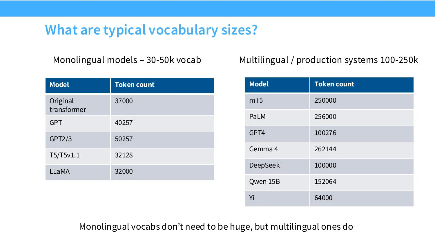
55:42 And then post-LAMA, a lot of people were really interested in multilingual or like production systems. So these include co-source models like GBD4. All these have much, much larger vocab sizes. And these are roughly in the 100 to 200,000 vocab range. And you see generally that, you know, Google models have a ton more vocab. LAMA derivatives roughly range at about 100,000 tokens. And then the sort of monolingual models are about 30,000. This is somewhat clear. The multilingual models really do need much larger vocab to cover the whole space. Generally, the models on the right #

56:17 are also bigger. There have been scaling law studies showing that the bigger your model, the larger the vocab it can handle. And so this is also partially driven by modern scaling trends, where the models on the right are generally bigger. No one's training small, sorry, large monolingual models anymore. Okay, so yeah. #

56:48 Sorry, the question was like, if you have, sorry, multilingual models or sorry? Multimodal. Multimodal. Yeah, so I guess it depends on the way that your tokens are encoded. But, you know, if you're tokenizing your images and things like that, then you need to, you know, have many more tokens to account for those. If you look at like various open source releases, they'll have like a different image tokenizer with its own vocab, which is quite large. Yeah. How valid is it to compare bits? #

57:21 How valid is it to compare bits? Oh, that is a great question. Okay, yeah. That's not a hyper primary question, but that is a good question. So what is the right way? Okay, so let me, let me like step back a moment and like put us in the right mindset. So if we think about language modeling, language modeling is a generative modeling task, right? We are modeling the probability of a sequence. Now, as long as your sequence is fixed, right, it's the same, you haven't, you know, adulterated it anyway, and you provide a probability over all strings, that's always valid to compare, right? At that level of things, it's always valid. Now, when you ask the #

57:55 question, is it valid to compare the bits per byte of arbitrary token, or two arbitrary tokenizers, tokenizers? Really, there's two things at play. The one thing is, you know, did you touch the sequence at all? Like if you look at some tokenizers in the past, before subword tokenizers, they would drop some tokens or drop some words. That changes, that makes the comparisons invalid. But modern tokenizers are complete, they can model any sequence, so that's not a concern. The other thing that you have to worry about is, are we like length normalizing in any way, right? But for bits per byte, you're always normalizing with the same number, which is the number of bytes, and so this is always a valid comparison, right? So that's kind of how to think about, you know, tokenizer comparisons. #

58:34 So, for example, I think they have some results. So is that comparing perplexity for fixed tokenizers, this always leads to. #

58:53 Perplexity and BPV are kind of dual to each other, so yes. Okay, that's what you're asking. It's only yes, it's only no, because if you're comparing, #

59:04 you could frame comparing the back perplexity as compared to BPV, but you're changing different things. Okay, we'll have to talk later, because I'm not sure I understand the question, but I think that's an interesting set of questions. Okay, good. Okay, all right. So, you know, we're going through really the lowest levels of details of language modeling, which I think has really exposed a lot of interesting ideas while we sort of talk through this, and I think dropout is one of the, and regularization, I think is another very interesting class of ideas, also one that I think is very counterintuitive from your machine learning 101 intuition. So, let's go through what I think is like the standard argument for, you know, regularization. Well, if I'm doing language modeling, I have a lot of data, right? I have more data than I can process most of the time, right? Unless you're at, you know, Google, maybe even then, there is more internet data than there is flops, so, you know, I'm probably not even going to see the same data twice, right? #

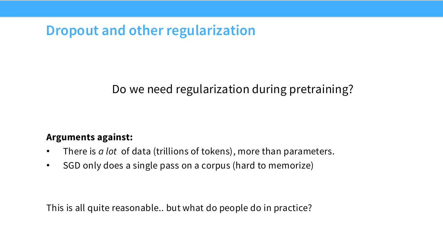
1:00:07 So, I'm only going to do a single pass on a corpus, and there's very good reasons and arguments to believe that a single pass of SGD or other optimizers is never really going to memorize my data very much, right? So, this means overfitting is not really a problem, almost ever during compute constrained language modeling. Now, you know, some people even actually only look at training loss because they believe so strongly that overfitting doesn't happen in single pass SGD. Now, given this, you know, you can sort of sit and think about this. Should I use dropout or weight decay in language model training, right? Okay, you can think about it a bit. You know, one unfortunate thing is that a lot of recent models don't talk about this stuff at all. It's really lower level details than, like, tech reports are willing to expose. But if you look, actually, you find a lot of models do both. #

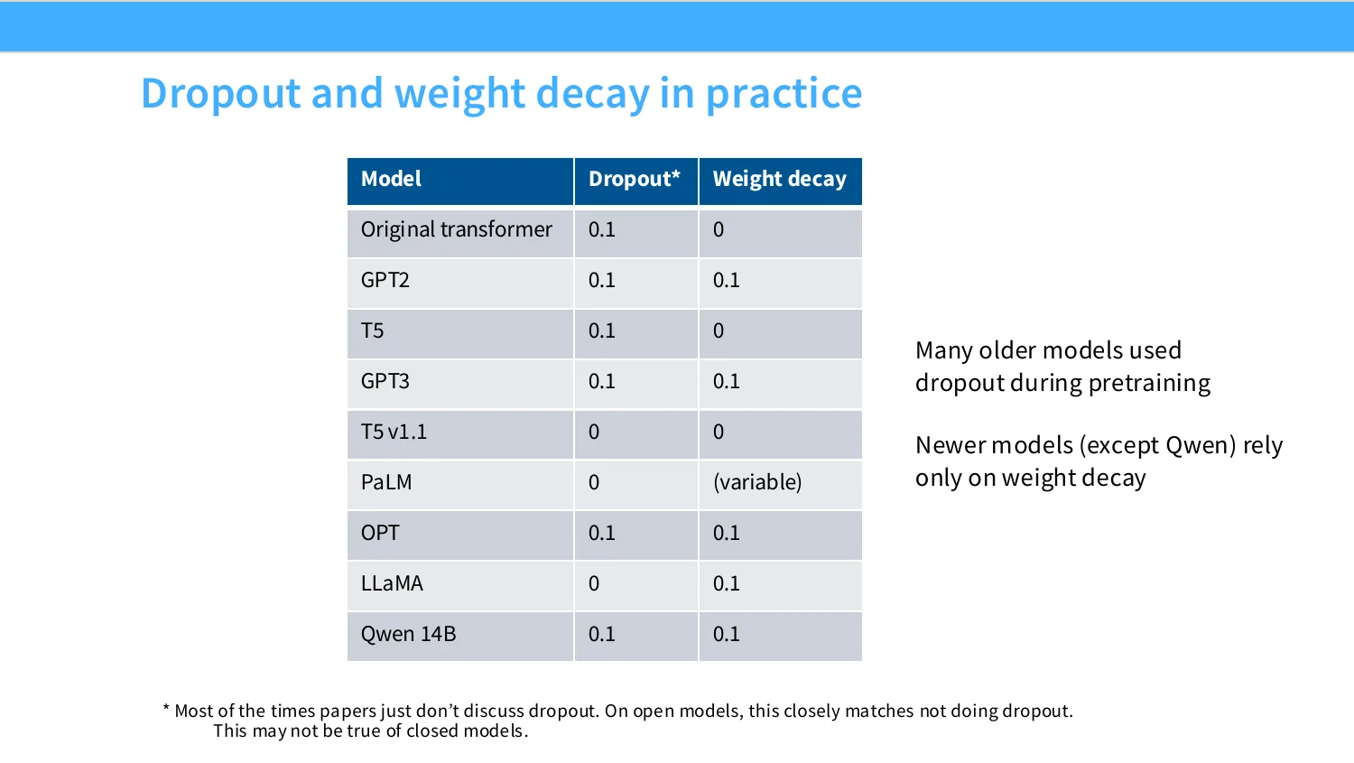
1:01:03 Especially weight decay, actually, is a fairly popular intervention even for modern high performance language models. This is very, very surprising. You know, I mean, some of the dropout things, you know, maybe have gone out of favor, but weight decay actually remains fairly popular. And this is very mystifying. Like, why is this? And this is, you know, one of the reasons why I think deep learning is hard and this architecture lecture is very strange and hard. It's because these things interact in very strange ways. So there have been papers that have argued and shown nice evidence that weight decay is actually not a regularizer sometimes. It actually interacts with the optimizer to essentially make optimization better. #

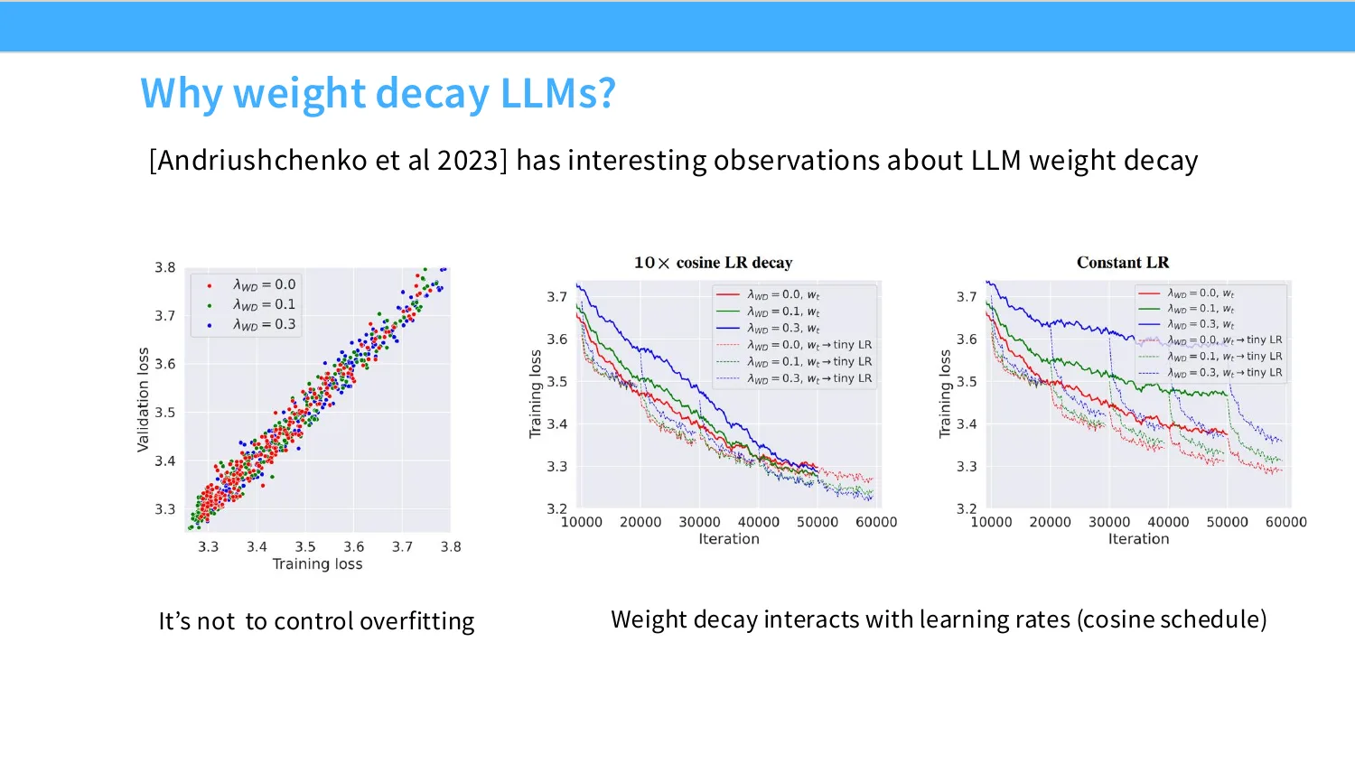
1:01:54 So if you look at the training versus validation loss across different weight decay settings on, you know, language model training for single path SGD, you don't really see any difference. Like, weight decay isn't shifting things so the validation loss is better. There's already no overfitting. We're on the x equals y line here, right? So it doesn't control overfitting. But if we kind of look at different levels of weight decay, and not only just different levels of weight decay, we look at weight decay combined with learning rate decay, what we find is that the stronger weight decay runs, these blue dashed lines on the bottom, you know, do significantly better because they start out slow, but they essentially end up converging to a much better minimum later. And this is, you know, generally true when we decay learning rate, not necessarily true when we're in constant learning rate, which is maybe somewhat more of where your intuition is coming from. So, you know, this is part of why it's very difficult to reason sort of a priori or like from scratch, you know, the behavior of all these different choices and why, you know, I think Percy and I have designed this class so that you interact with stuff, because, you know, you might come upon this thing that we're basically, weight decay is actually an optimization intervention and not necessarily a regularization intervention, which is, you know, what you would expect here, right? So always keep that in mind that these kinds of unexpected effects can really start to kick in for these kinds of settings. #

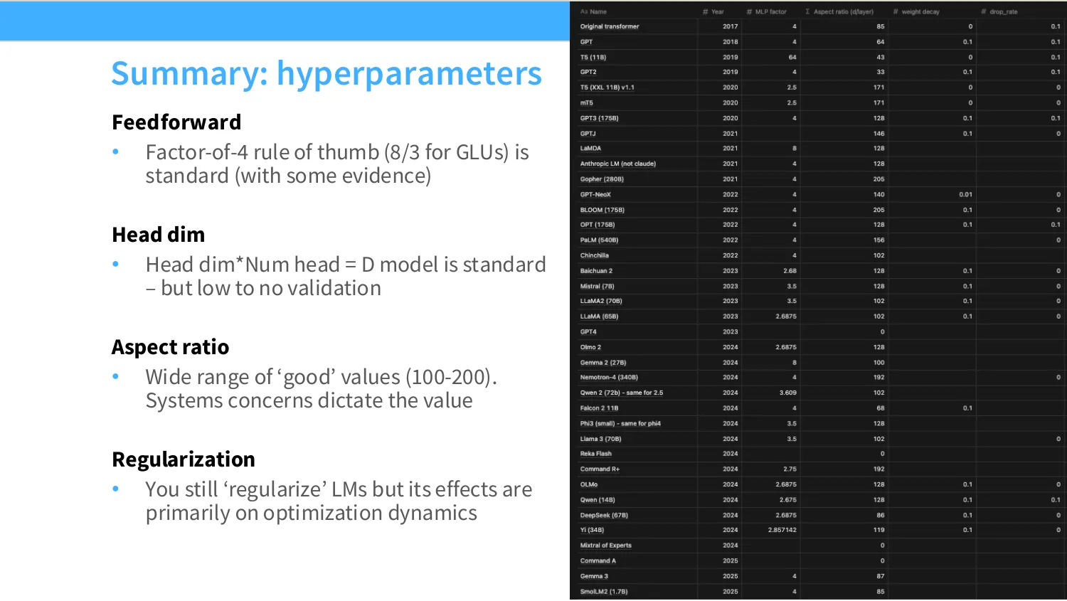
1:03:23 Cool. All right. So to put everything together for hyperparameters, there's actually for, you know, a lot of the maybe more hairy looking hyperparameters, actually just fairly standard choices that have worked well for everybody, right? You know, factor a four rule of thumb, keep your head dim and your number of heads equal to the model dimension, pick an aspect ratio roughly around 100. And, you know, if you ask about regularization, right, you want to maybe try a couple of things, because regularization actually does interact with optimizers in ways that are quite counterintuitive, right? So this is the thing that some people still do, even though you don't need the regularization at all. Actually, maybe I'll stop here. Yeah? Are there any architectural differences maybe for like the diffusion model? #

1:04:12 Ooh, diffusions. That I have not looked into enough, to be honest. There aren't that many people training big diffusions is one issue. And many of the models that have been trained are retrofitted. So I think the architectures are actually the same as the, you know, like a Lama-like model. But if you're asking the question of like, what's the optimal architecture if you were to train from scratch, I don't know what that is actually off the top of my head. Yeah? Do you have an explanation for why regularization must affect optimization? Well, I guess it's not that regularization in general affects optimization. #

1:04:42 I don't think people do dropout anymore because, you know, it doesn't really interact well with optimization. But for example, weight decay, you know, which is shrinkage to zero, that might allow you to use a higher learning rate or it might allow you to decay faster. There are lots of ways in which all of these terms are interrelated. #

1:04:59 Cool. Okay. #

1:05:01 Now, I've talked a lot about how to design expressive models by sort of looking at all these other models that have been trained. #

09 训练稳定性技巧：z-loss / QK-norm / Soft-capping

1:05:10 One of the things that I'll highlight now is over the last few years, a really big emphasis has not been on performance alone. It has actually been on stability. And this becomes an increasingly important concern as your models get more and more expensive to train, right? We've kind of seen that a lot of these choices are forgiving, right? Everyone's kind of doing similar stuff. And so, you know, you can mess with these, but you're not going to get a big performance difference. That's fine. But if your model, you know, suddenly blows up some part into training, like you get these horrible looking spikes all over the place, you know, you might end up with a model that is, you know, actually not very good quality, right? Or it might be unrecoverable. #

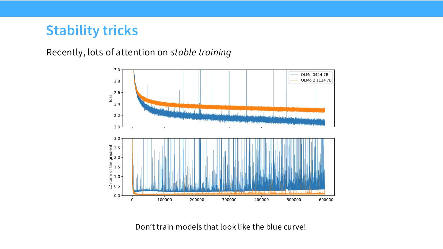
1:05:49 You might have spent, you know, millions of dollars in training, and, you know, you get to a point where the model is no longer able to be trained any further, right? That would be a horrible thing to happen if you have a lot of compute that you want to spend. So you don't want to train models that look kind of like this blue curve with, like, spikes everywhere and these, you know, big gradient norms happening. So what do we do to fix these stability issues? I mean, this is really, I would say, like a core, core issue. And, you know, if you have stability issues in language models or in general neural networks, there's a few, you know, usual suspects that you've got to start looking at. One of them is the soft maxes. And the soft max has two things that are both really bad for stability. One of them is an exponential, right? #

1:06:32 You can see how that blows up very quickly. You also divide two numbers, and that's also a potentially very dangerous operation, right? So a soft max is one place where you've got to be extra, extra careful. And where are the soft maxes in a language model? Well, there's two of them. There's one on the output side when we output our probability distribution. And then in attention, when we normalize the attention, there's going to be another soft max, right? So we can think of both of those as really kind of danger zones for our model, especially the attention. #

1:07:05 But okay, let's start with thinking about the output soft max. The output soft max can blow up on us. And one of the things that we can do is we can try to control sort of the normalizer problem. So, you know, let's sort of think about the soft max calculation. We want to compute a log probability to compute the loss. Now, what is the log probability? Well, it's, you know, the output of your model, u. And then you've got this log normalizer, right? This u is well behaved because in some sense this is the output of your model, right? #

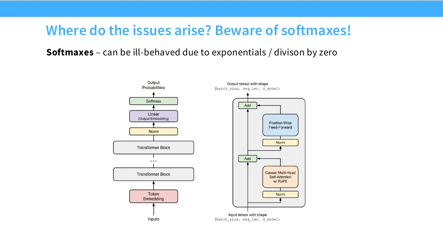
1:07:36 This is just the output of your residual stream with all the things that are added in. So if u is well behaved, then log p, the first term is well behaved, right? If the model is being okay. Now, the second term, this log z, this might not be so okay, right? If z is really big or really small, even if the output of your model is somewhat well behaved, it could blow up. And what is z? Well, it's an exponential, right? So it could potentially blow up very quickly on you. Or if this is zero, it could also blow up on you, right? #

1:08:02 So both of those directions are very, very bad. Now, we would ideally like our z to be somewhere near one, right? Or log z to be somewhere near zero. What can we do? Well, one of the things that you notice, right? If you sort of thought about the action of the softmax, is this whole thing is over parametrized, right? I could sort of push things in and out. So if I add a constant to u, I can manipulate the z's without really affecting the output of the softmax, right? It can cancel out between the normalizer and sort of the output of my model. #

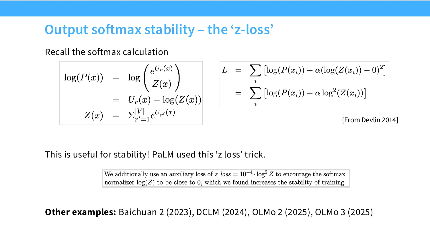
1:08:35 So because of that property, one thing that I could do is I could add a regularizer. This is from Jacob Devlin's paper, 2014, in which he adds sort of this squared log z term. And what this is doing is it's just penalizing how far away your log z is from zero. And if log z is near zero, that's nice because this whole expression is kind of numerically stable. This is called the z loss trick. It's been used by a number of papers. Jacob Devlin and others sort of popular or initially pioneered this back in 2014. And then it's become popular again through a number of open source models. Like, Bychuan, I think, was the first open source model to do it. #

1:09:18 But then DCLM and Omo and others have been using this trick to stabilize their output softmaxes. So this is a surprisingly effective thing. Now, okay, so let's say we've handled the instability issues on the output softmax. Now we have to sort of turn our attention towards the other potential problem, which is attention, right? And this is a place where lots of degeneracies happen. Lots of techniques have been developed to control the instability that attention operations generate. And really the high level thing that I'll say is if you have instability, if you can throw a layer norm in there somehow, it might control it. And that's really in some sense the design philosophy behind this idea called the QK norm. So what you do is remember that we have our Q's and K's that are going to be multiplied together. #

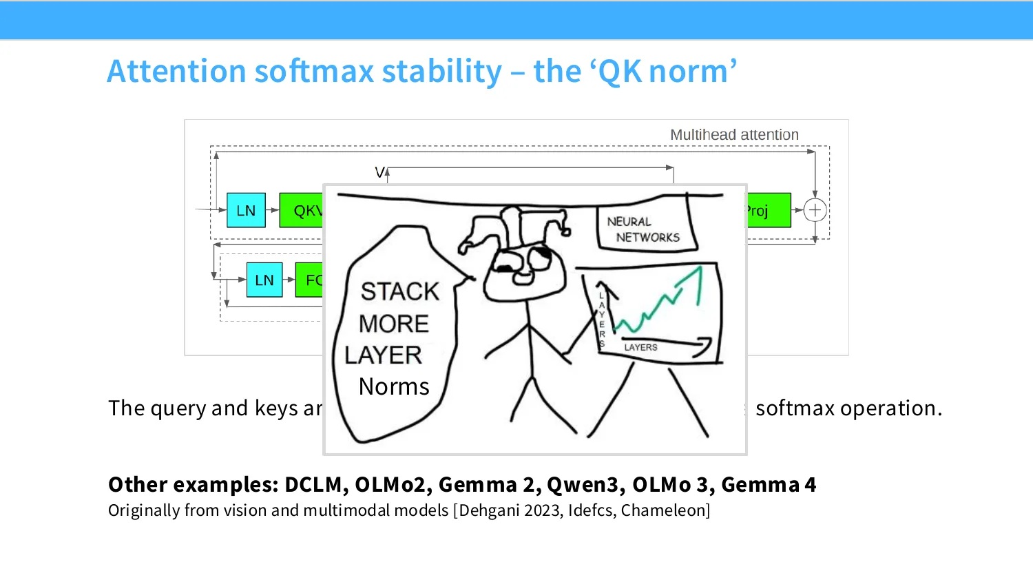
1:10:11 And then they're going to go into the softmax, right? So in the standard attention operation, I'm going to layer norm as a pre-layer norm, multiply with a QKV, and I'm going to get my Q's and K's. Those will get multiplied by a matrix multiply. I'll softmax them, and I'll multiply that with V to get the weighted average, and then I'll output whatever comes after, right? So this is our usual attention. Now what happens if we just throw in a layer norm before we multiply the Q's and K's? If we do that, then we know that the inputs to this matrix multiply, and therefore the inputs to the softmax roughly have the same scale. They're always going to have a scale of roughly one, because we've used RMS norm to divide the size of those Q's and K's. So if we do that, then we're kind of going to keep this softmax operation stable. #

1:11:00 Tons of different models do this. It's originally from the multimodal world. Some folks who were making multimodal models sort of initially discovered QK norm. Edifix and Chameleon really used this and proved it out. And then a number of other open source language models realize that the same tricks are entirely applicable to stabilizing attention for language models. And I think this is now very, very standard. Like QK norm is actually a very standard intervention that most of the large models now introduce. It doesn't seem to affect performance from lots of different training runs, but it does definitely prevent the kinds of attention degeneracies. And you know, I'm really, the way that I've seen this is, you know, we have layer norms initially in the pre-norm. #

1:11:50 Now we add them after the non-linearities in each block, and now we're throwing them in both the Q's and the K's. And really, I think this is kind of getting at the stabilization tricks that people apply to this rule. Okay. Now, the final set of things that I'll talk about as a stability intervention, and frankly, this one is not as popular and more of a Google specific trick that I've seen. But logit soft capping is a much harder intervention that some people apply. So this one, you know, in QK norm, what we're doing is we are controlling the inputs, the soft max, and sort of hoping that the outputs are well behaved. If we really, really want to enforce well behaved outputs, what we can do is we can kind of take the logits, the things that go straight into the soft max, and we can just cap them off so they can never be too large or too small. Right? This is almost a hard constraint. #

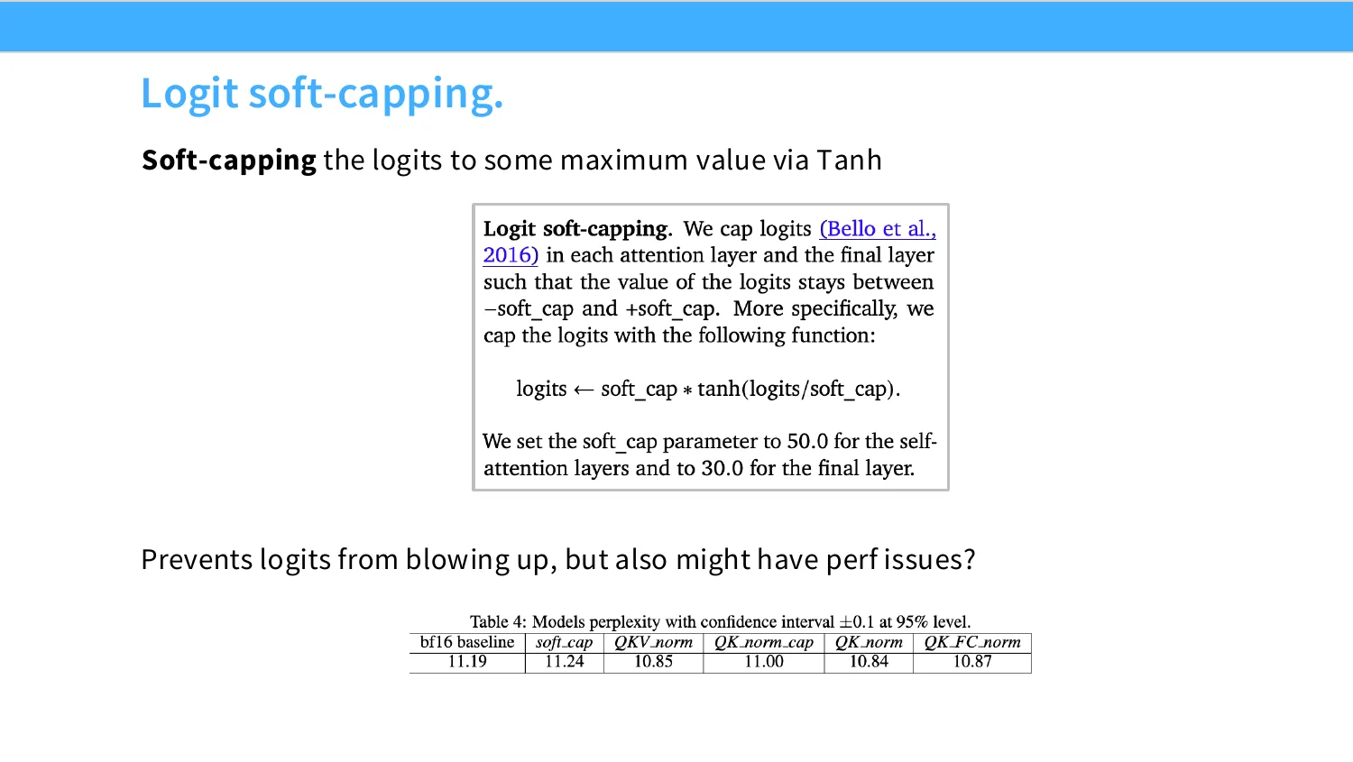
1:12:45 It's called a soft cap, of course, but a tanh, you know, is bounded at some value. And so this is in the gamma models. I think both gamma or like gamma 2, 3, and 4 all use the logit soft cap trick. And what they do is they take all of their logits for the attention layers, and then they soft cap them at some value. Some NVIDIA folks have done actually quite nice work doing systematic comparisons of these stability interventions. And what they find is if you start with a baseline model, you can do all sorts of different interventions. And QK norm is here, and it does slightly better due to the fact that you can crank up the learning rate a little bit. But if you do soft capping alone, you actually end up losing performance. So there is a quality degradation that happens. #

1:13:35 This is a very strong intervention. You can never express very confident signals in your soft max beyond a certain point. #

10 注意力头变体：MQA / GQA

1:13:41 So it does have some negative consequences, but this is a very safe way of stabilizing the outputs of your attention. Or sorry, the inputs to your attention, the logits that go into the soft max. OK, so that's kind of the end of the stability components. I can pause for a moment here, and I'll talk about sort of various attention things after that. #

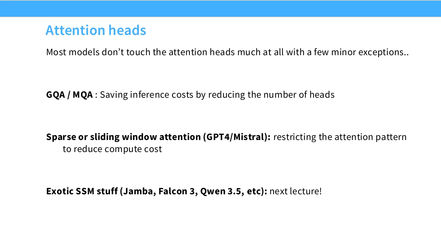
1:14:06 Cool. OK. All right, so the last thing I want to talk about today is various interventions that you can make your attention to. And as I was saying at the beginning of this lecture, I'm only going to talk about all the things that you can do to sort of dance all by all attention today. So if you were interested in hearing about state space models or linear time attention, sadly today is not the day for you. The things that I do want to talk about, which are really commonly implemented attention interventions today, are group query attention, which really saves inference costs by reducing the number of heads. And sparse or sliding window attention, which really originally came from the GPT3 family, but have now really been adopted widely by most models that are looking to do long context, unless they are doing exotic SSM stuff. #

1:15:01 So I'll start with group query attention or GQA or MQA. This, I'm going to first set up the need for these kinds of things, and then you'll kind of hopefully see what the trick is and why it's fairly natural. So for the moment we've been talking about training and modeling and all these things, but let's take a pause, and now let's think about deployment. You've trained this very big model, and now you need to serve it to lots of users, and you're going to pay a cost for serving. And you're going to have to, in an abstract sense, pay for two different resources. You're going to have to pay for your flops, the computation that you perform. But you also have to pay for another thing. You have to pay for your memory accesses, because the memory accesses are also going to impact your system's characteristics, your latency, your utilization. So you want both of these things to be small. #

1:15:53 Now, let's think about what happens during training, or alternatively, pre-fill, when you're looking at your prompt where someone gives you the stuff. In this case, the total arithmetic operations you have is order of magnitude, batch size, sequence length, hidden dim squared. That's roughly the size of things that you get. And of course, we're doing quadratic attention, so we've got d squared. #

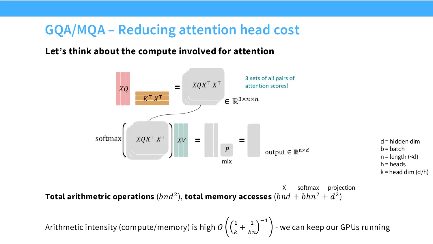
1:16:17 We've got total memory accesses, like what is our memory access that we have here? We have batch times sequence length times hidden dim, plus the sort of cost of the softmax, which has an n squared component. And then we've got a d squared component for the projections. So the arithmetic intensity here is pretty good. It's going to be 1 over k. This is the number of heads, so you need to have, sorry, head dims. So your head dims need to be big enough that you're multiplying some reasonably sized matrices. And you've got a 1 over bn, so your sequences need to be long enough, or your batch sizes need to be big enough. As long as both of these are true, your GPUs are going to be fully utilized. #

1:16:55 Great, you're using all of your resources. #

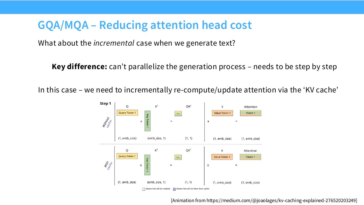
1:16:59 Now, you know, we have finished training, and now we're serving our users. How do we serve our users? We're going to generate tokens and send it to them, right? Now, if we're doing that, I can't parallelize the generation process. What I'm going to do is I'm going to generate a token. I'm going to condition on it. I'm going to generate the next token, and I'm going to repeat this process one by one. This is just sort of the curse of autoregressive language modeling. We have to do this. #

1:17:23 In order to do this, the efficient way to do it is to maintain all of the sort of past keys and queries that I've had in what's called a KV cache. So the KV cache is going to maintain this matrix of, you know, Q dot K over the past. And then whenever I need to compute something new, I can reuse sort of the sub matrices that I've already had from the past. And I only really need to compute sort of the new query key interactions that I need to fill out the rest of this matrix, right? So every sub matrix I've computed before I can keep. I only need to compute my new one. So this saves a lot on compute, right? That's great. #

1:18:03 But the issue here is now our arithmetic intensity is not so good, right? As you might sort of intuit, this KV cache approach is going to be reading parameters all the time, right? Each time I have a new step, right, I'm going to have to read in my parameters. I'm going to have to take these dot products. And I'm going to do this once every step. And so now what do I have? Well, you know, my total memory, sorry, my total arithmetic operations are the same. I'm multiplying the same matrices still, right? Just incrementally rather than all at once. #

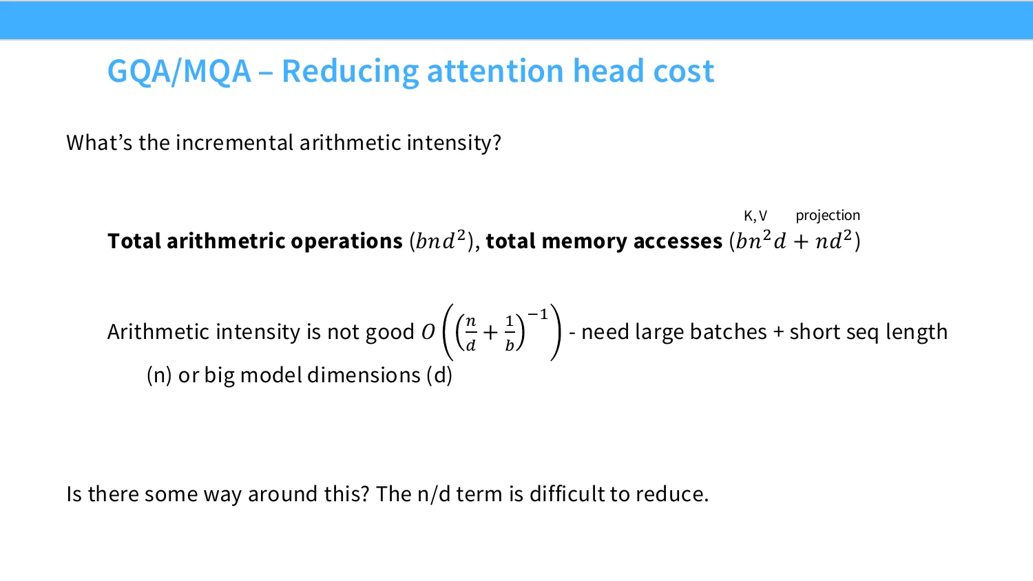
1:18:34 But because I'm doing this incrementally, you know, now I have a memory access pattern of batch by sequence squared by hidden dim plus sequence by hidden dim squared. And the second term is not so pleasant, right? It used to be that it was just d squared, but now we've got n times d squared. And if we compute the arithmetic intensity, which is the ratio of these two guys, now we have n over d plus 1 over b. So now what we need is large batches plus short sequence length, or we need really big model dimensions. So if we want to serve a small model efficiently, this is not so good, right? This is really difficult to deal with, right? This n over d term, this first term over here, which is sequence length over hidden dim, is very difficult to reduce if we're doing this incremental computation. This is just a hard thing to deal with. #

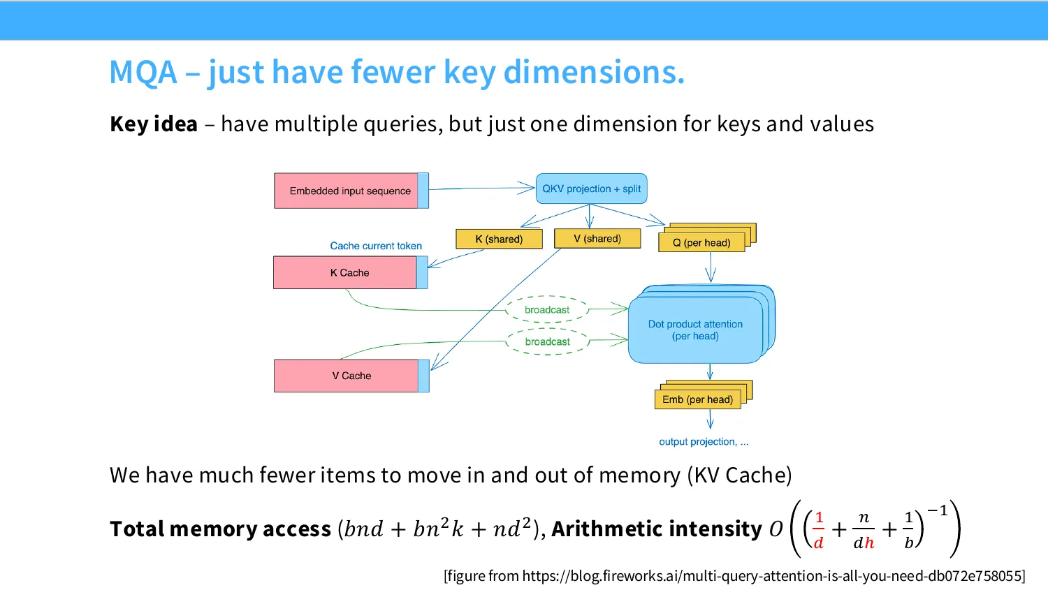
1:19:32 So this leads to this idea of MQA, or multi query attention. Normally you have multiple heads in your attention operation, and you're going to have different keys, different values, and different queries. That's normally how you do things. But one thing that we could do is maybe we can keep the k's and the v's the same across all the heads. And the only thing that's different across the heads are the queries. If we do this, then this drastically removes the amount of items that need to be moved in and out of memory, right? Because the kv cache, right, are now significantly smaller. These are all shared across all the heads. This significantly reduces the total memory access as well as the arithmetic intensity. #

1:20:14 And we're kind of, the key term that we were talking about here, we had the n over d term. Now we have h multiplying this, right? And so this h term allows us to significantly reduce the, sorry, increase the arithmetic intensity if we have a lot of heads, right? This is a significant gain over what we had before. So this gets us significant efficiency improvements. But the issue with MQA is, this is on the right here, you have one value and one key for all these queries. You do in fact lose significant expressive power if you do this. And so there's this trade off between systems efficiency and expressiveness. And you might wonder, is there sort of a sweet spot in which we can avoid trading off, you know, quite as significantly expressive power and computation. #

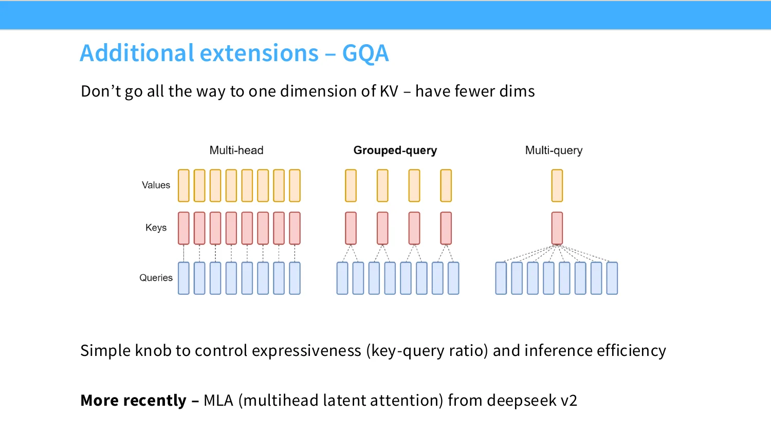
1:21:07 And that's where GQA or grouped query attention comes in. You know, the original transformer is multi head. We have queries and keys for each head. In multi query, we have one key and value for each, for all the heads. In grouped query, we reduce the amount of keys and values, but we keep the number of queries the same. So we now have this ratio that we can play with, which is kind of the number of key heads or the number of value heads, while keeping the total number of heads much larger than that. So this allows us to very simply control the trade off between expressiveness and inference efficiency. There are other sort of tricks from deep seek V2, multi head latent tension, that I'll sort of mention briefly next time, which sort of have a different kind of factorization structure and a different set of trade offs. But really, the nice thing about GQA is that in practice the trade off is quite favorable. #

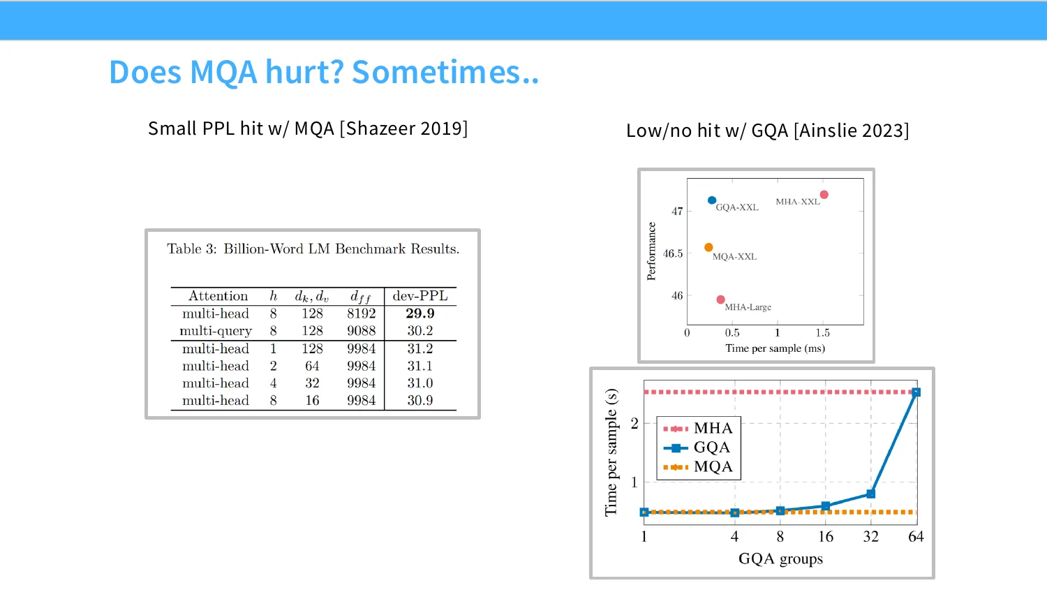
1:21:59 So if you have multi head, your performance, this was, you know, in the, I think, T5 days, if I remember right. This is your downstream model performance. This is your time per sample. You want to reduce this as much as possible. With multi head attention, you have best performance, but very high cost. With MQA, you know, you have lower cost, but much lower performance. Similarly, if you make your model smaller to try to hit your performance target to get much worse performance, GQA really does get the best of both worlds. You know, very low inference cost, nearly the same performance as your full multi head. And you see sort of this like GQA group structure where if you have a small reduction in the number of heads, you basically have most of the gains in your performance, which allows you to sort of keep most of the expressive power while getting significant inference improvements. #

1:22:54 And first you'll talk a bunch more about sort of the inference mechanics later. But sort of this should give you a flavor of like why models today almost all adopt this GQA structure, because it gives you a lot of this inference cost, which is really critical, without very much of a expressiveness hit. #

1:23:14 Cool. Any questions for GQA or KVCache? Yeah. #

1:23:20 But given that you have so many rules of terms for what hyperprimes are good, like do one of them still searching over hyperprimes versus exploiting these rules of terms? #

1:23:33 I think it's a mix of both. I think every sort of model training run has some theses about what can be varied. And so you see this in a lot of the reports where I think the hyperprimeters are often not where people are touching too much. But you see like architecture changes like one at a time in a lot of these reports. But it's very rare to like go and change everything up. I think Google is one of the only orgs that seems to like really spice things up in a significant way. The gamma series has done some pretty interesting things. The most recent gamma 4 release, for example, now has like individual embedding for every layer in a way to control the tradeoffs between like memory use and flops. It's a very interesting set of things that they've done. #

1:24:14 Oh, yeah, back there. Have you ever done experiments with like dynamically altering some of these parameters during fading? During fading. Let me see. #

1:24:26 Weight decay. Yes. Weight decay. People change in concert with like learning rate. That is actually a heuristic that people do. That works very well. Other than that, I don't know if there's a lot of different hypers that people change during training, especially because the architecture ones just make training incompatible. So you can't really change them while you're training. Yeah. #

1:24:49 So I think I think weight decay is probably the one that I can think of. The others are usually fixed. Yeah. Yeah. #

1:24:58 It's not just inference time. It's a pleasure. That's right. Yeah. You train with a certain number of keys. #

11 稀疏 / 滑窗注意力与交错策略

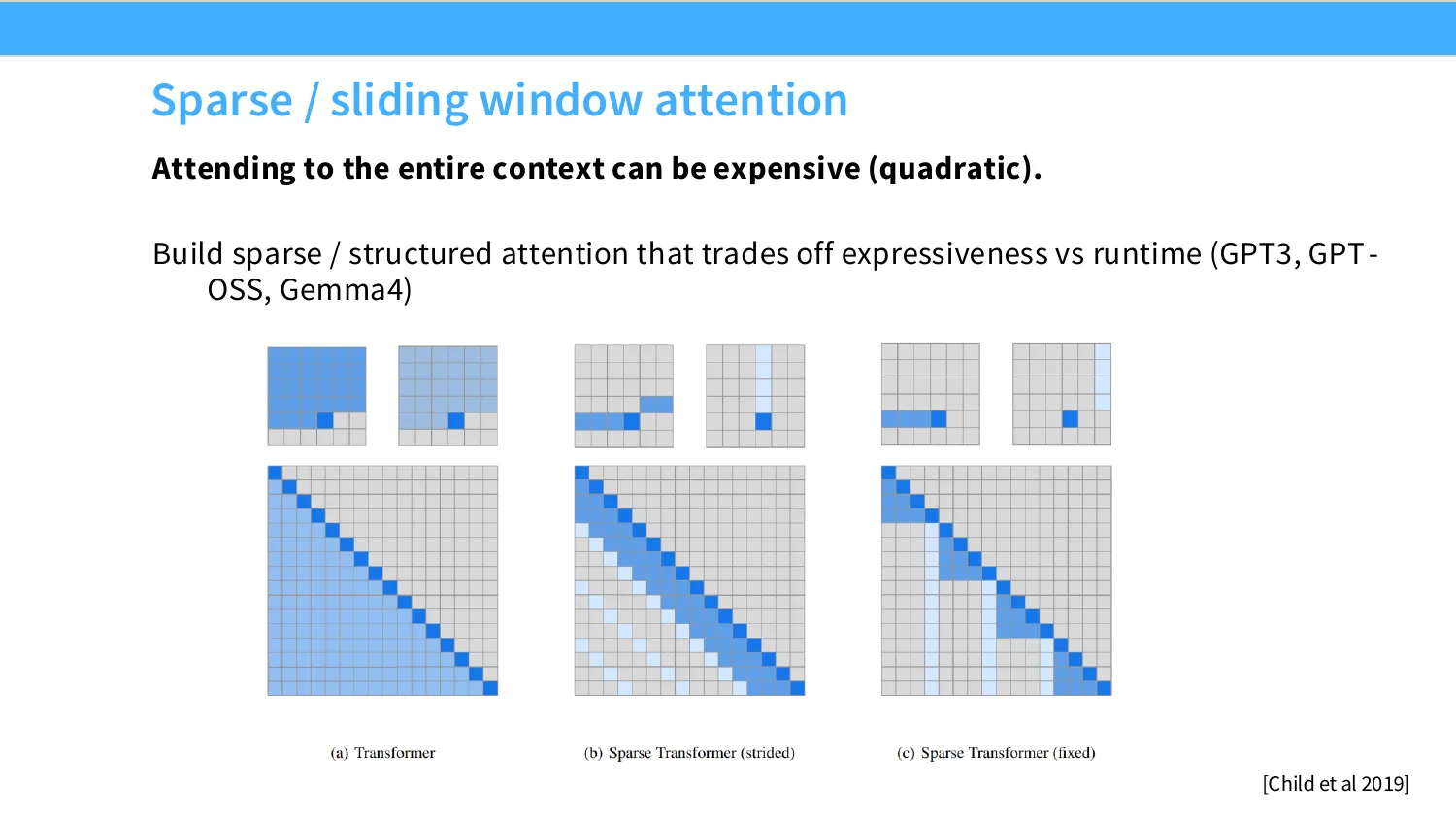
1:25:08 Okay. The last thing I'll talk about is sliding window attention, which is a really old idea. Like, you know, GPT-3 used actually this, you know, if you read the paper, they'll say we alternate between full attention, which where every position can attend to everyone in the past, and a banded matrix style attention where you can attend to everyone within a fixed window. And, you know, open AI has some early work on these kinds of like different kinds of attention patterns that you can use. But actually this has become really, really popular over the past year. This idea of alternating, you know, the big full attention and a more local attention actually hits a sweet spot for how to manage like long context performance while not paying too much for inference. #

1:25:56 I think, you know, the more recent revival in open models, I would maybe say, here command A was the first one I saw do it, where they, you know, had this like structure where every four layers they would have a full attention that attended to everything. The three layers in between would use a sliding window attention that would only be able to look at local structure. And of course, you know, as you go up, sorry, in this case down because they ordered the diagram the other way, as you go down sort of these blocks, you know, you're aggregating local information into global ones. The local attentions at the end can, of course, access more global information. But this, you know, allows you to manage the cost of having a really long context without having to go for something like a state space model or more exotic intervention. And that's worked quite well. There's also some innovation where people change the embedding format for the long range information where they get rid of things like rope. So you have no position embeddings at all. So you're really looking almost at bags where the short range information still gets position information. #

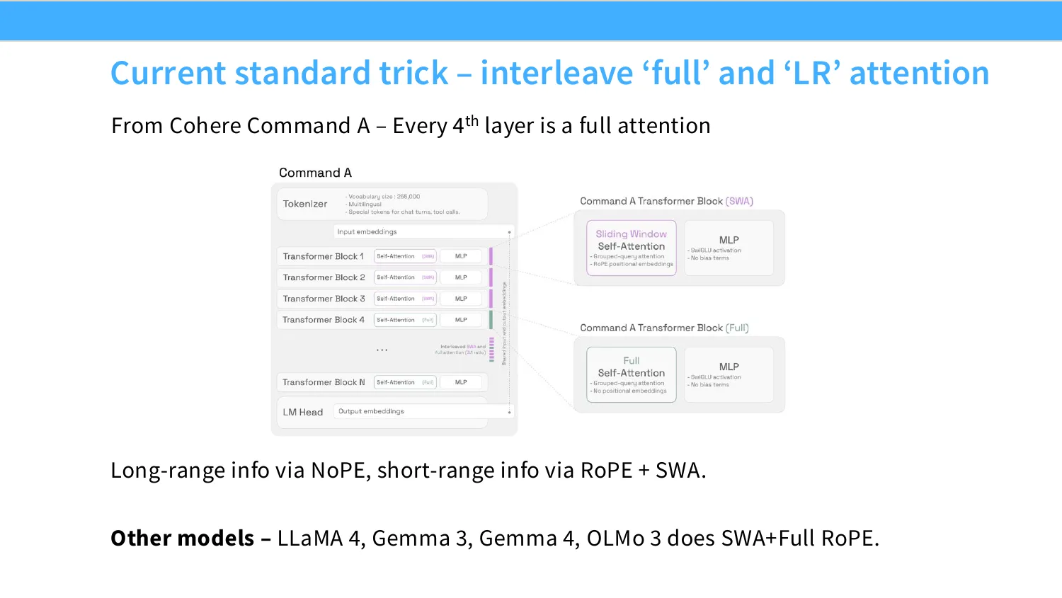
1:27:02 So people do all sorts of, you know, kinds of interventions involving these both embeddings and alternating local and global structure. I'll say that this is a, you know, attention and in general how to manage the tradeoff between long context and sort of long context cost and performance is still an active area of investigation. It's a place where the most architecture work and changes are still being done. We see essentially a bunch of other models adopt this idea. LAMA4, most recently GEMMA4, OMO3. They all do this combination of sliding window attention and full attention. In their case, using full rope instead of NOPE as the embedding. So as I said, this is becoming really, really popular. QEN 3.5, which I put on the right, they're actually a little bit different because they alternate a state space model called gated delta net and a full attention every sort of, you know, one full attention every four layers. #

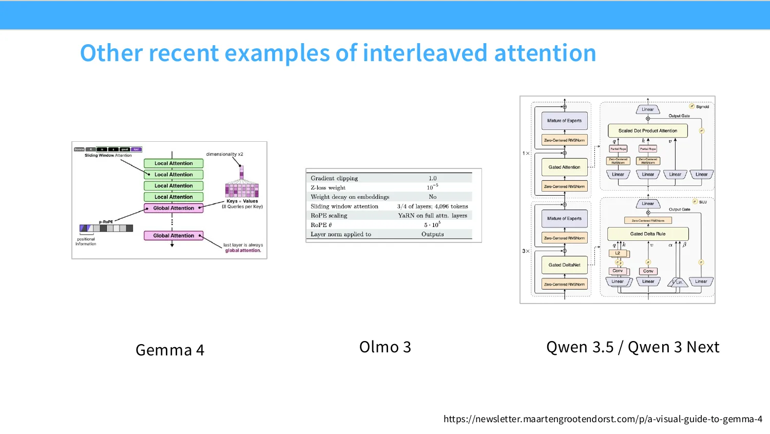
1:28:04 So it's the same alternating structure, but they're using a different sort of cheap layer. In their case, they're using a state space model. I'll explain what that is next lecture instead of a sliding window sort of local attention. But you see, this is like, I think, a new theme over the past year where, you know, open models are really trying to grapple with long context performance. And the way to do that, at least so far, is to have these hybrid models that aren't just global attention, aren't just cheap attention. There's some sort of mix in between. #

12 总结

1:28:31 And that seems to have worked very well so far in a lot of these models. #

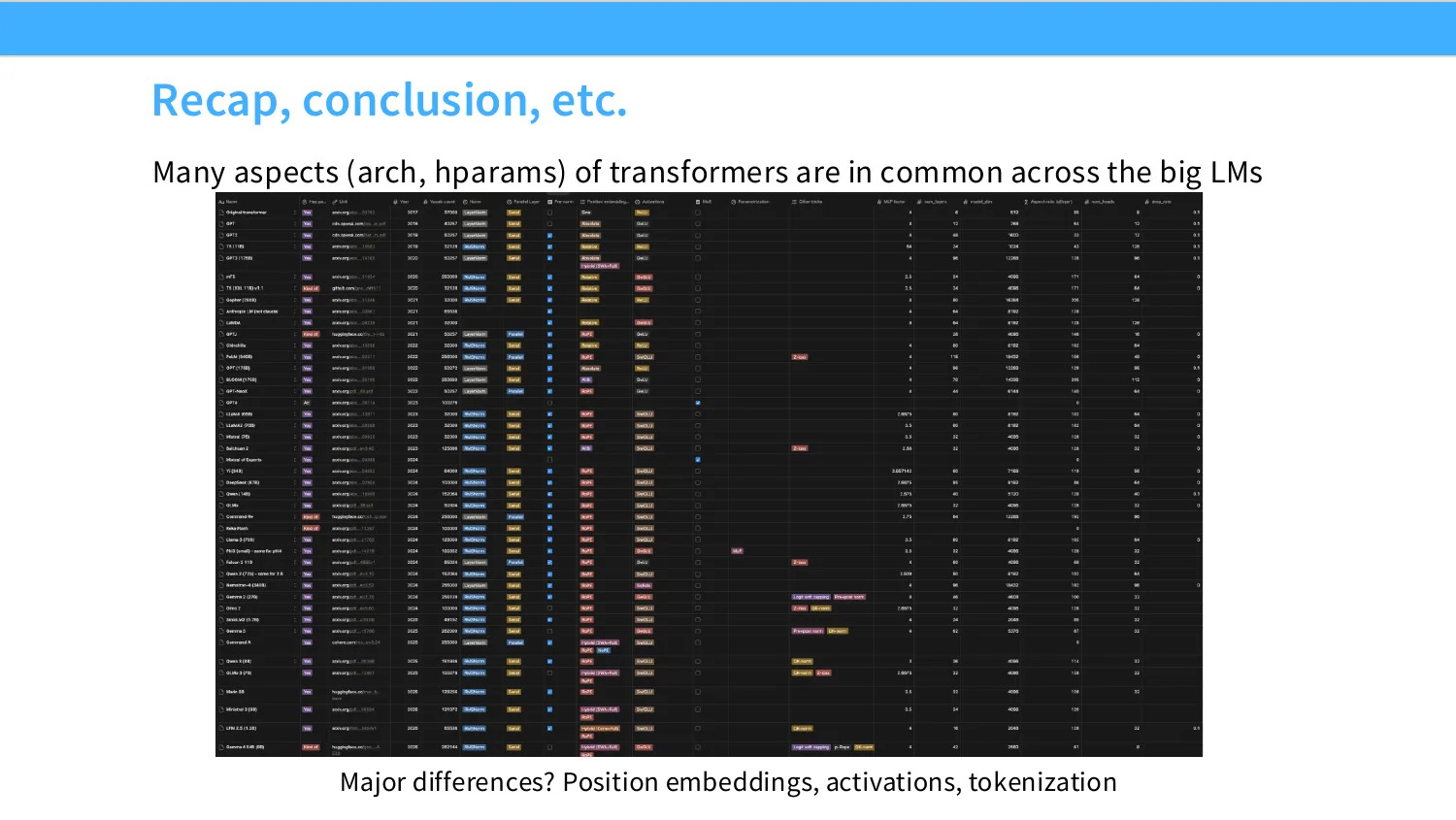
1:28:37 OK, cool. So as I was sort of trying to emphasize, when you look across all of these models, you start to see a lot of patterns and hopefully a sense of general understanding about what things you can do and what things are good defaults. We also see a lot of differences in how we handle context and how we handle position embeddings. Even tokenization, there's some differences, right? So there are differences across these models, but there's also commonalities that hopefully now give you some intuition as you go out and do your assignments and sort of mess with the leaderboard and so on. Thanks. #