并行
本页 = 官方讲义截图 + 全程文稿(whisper large-v3-turbo 转录,已去除语气词)
01 课程引入:从单卡到多卡并行
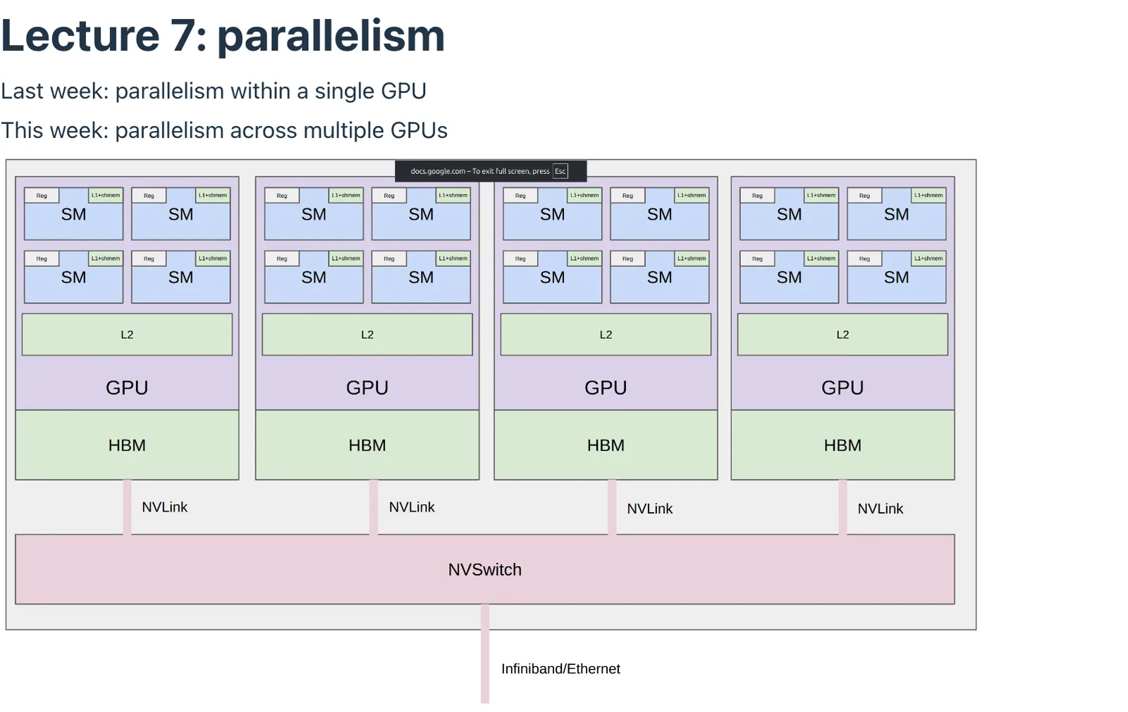
0:05 Okay, let's get started. So welcome back everyone. So today we're going to talk about parallelism. And remember in the last week, we introduced how to make a single GPU go fast by writing kernels, and we really looked inside this GPU. And this week, we're going to talk about how to leverage multiple GPUs to make your code go even faster. So the picture you should have in your head is something like this. So for the last week, we focused on one of these boxes, where you have your GPU. Remember, you have your high bandwidth memory, HBM, L2 cache, L1 cache, registers, and a bunch of streaming multiprocessors. So now the picture gets extended because instead of having one GPU, you might have four, you might have a thousand GPUs, and those are going to be connected.
1:00 And I'll talk later about how those GPUs are going to get connected. And then you're going to have to figure out how to leverage all of this compute, to train models.


1:12 So in both cases, meaning both in the single GPU case and in the multi-GPU case, as we'll talk about today, the situation is kind of similar if you zoom out, which is that the compute, the arithmetic logic, units, the tensor cores, so on, is far away from your data. And far away from a single GPU means all the way over here in, HBM. And, now if you have multi-GPUs, the thing that you need here might be all the way on a different GPU. And you're going to have to shovel, that over somehow. But the same principles are going to be the same because the game is to orchestrate the computation to try to avoid data transfer bottlenecks. It's very easy to use a ton of GPUs, but it's hard to use them effectively. So, taking a little bit of liberty, we can think about the generalized hierarchy where at the, at the sort of local level next to the, the SMs is a single node, single GPU, where you have, an L1 cache shared memory. This was the fastest. And then you had, HBM, which we lamented was so slow.

2:25 But in this lecture, HBM is going to be considered fast. now we're going to, think about the single node multi-GPU setting where the GPUs are going to be connected via MVLink and MVSwitch. and then finally the multi-node, the multi-GPU where we have to resort to infinite band and, Ethernet depending on what, network you have. Okay. So, last week, we talked about various, tricks for, imp-reducing memory accesses, fusion and tiling. Read into shared memory, do everything you, as much as you can, and then write it back out. and this week, we're going to talk about how you can reduce amount of communication, across, GPUs by, replicating and, and sharding appropriately. So, so why do you do GPU, multi-GPUs? the, the obvious answer is, well, you want to scale. But to put a, finer point on it,

3:26 there's really two reasons. One is that your parameters or activations or gradients and optimizer state don't fit on the HBM memory of, a single GPU. So, B200 adds 192 gigabytes. If you're training a one trillion parameter model, that's not going to fit on a single, GPU. And the other reason is that even if your model could fit on a single GPU, you might want to leverage more GPUs by, splitting everything up to train faster. So, sometimes there will be, kind of, some decisions to be made because, you, you could fit everything on GPUs, but you have fewer, cores. but if you spread out, then you're going to have to pay the communication bandwidth. Right? So, that's some calculation you're going to have to do to figure out, how to parallelize. Okay. So, just one note here is that, so far,


4:22 this lecture is Python. You execute it and you can just show everything. Now, this lecture, if you run this directly, it uses multiprocessing, s- but when I trace through it, I'm putting in some sort of, like, special single process mode. So, if you want to see the standard out for this lecture, re- run in the multiprocessing setup, you can click here, and I'll show this, as we go through the lecture. But just remember, as we step through this lecture, we're not actually doing multiprocessing, because we're just stepping through, single lines of code. Okay. So, this lecture is going to include, two parts. One is we're going to learn about the building blocks of distributed communication and computation, starting with the, program, a model, talk a little bit about the hardware, start to implement things in Torch, which you're going to, do on your assignment two. And then the second part is we're going to look at actual, training.

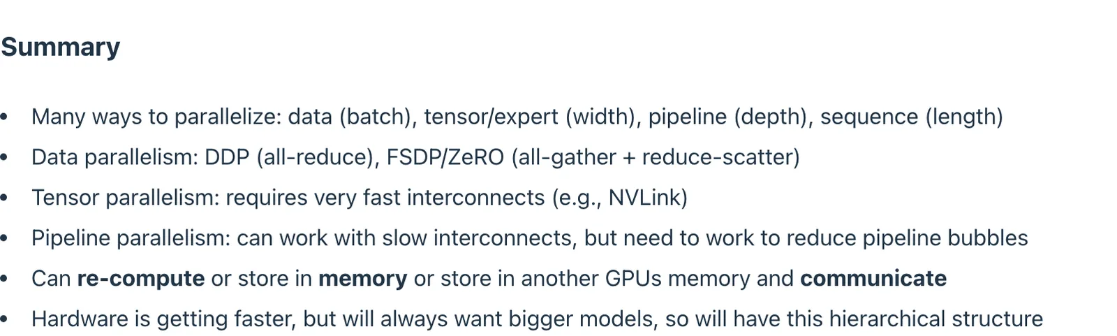
5:24 we're going to look at three types of parallelism, data parallelism, tensor parallelism, pipeline parallelism. Each is going to cut up our model in different ways.
02 集合通信原语:Broadcast / All-reduce / All-to-all

5:34 We're going to do this for, MLPs, rather than the full transformer, but it's really, sort of the core computation is going to be, shown here. Okay. So, let's dive in. So, the first thing to talk about is these things called collective operations. So, collective operations are these, primitives from distributed programming that go back to the 80s. So, the idea of parallel programming is, is very old. it wasn't invented for LM training. and it's still the case that these primitives are the ones that we, use, today. Okay. And here, collective just means that you're specifying a general communication pattern
6:22 or a template across multiple devices rather than managing, point to point how this GPU is going to communicate with another GPU. And this is going to be much, easier, and the system can do a lot more work for you. So, this is, a very tried and true interface for doing parallel, programming. Okay. So, the general setup is as follows. the terminology here is a little bit, I find it a little bit strange, but this is standard and, parallel programming. The idea is that you have a bunch of ranks where rank corresponds to a particular device. In our case, a GPU could be a TPU. But the point is that you have, let's say, four ranks here.
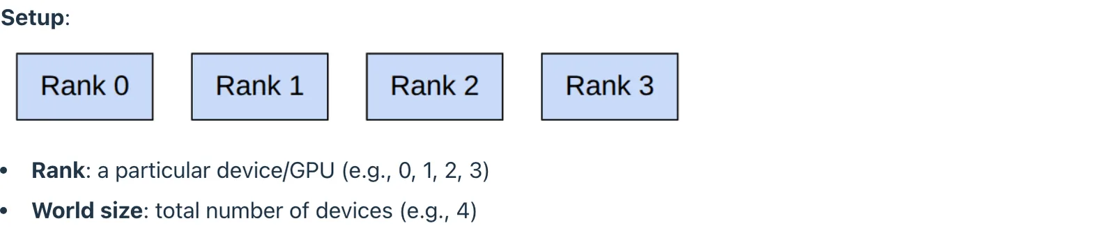
7:06 The world size corresponds to the number of devices. So, the world size here is four.

7:12 Okay. So, there is a few operations we're going to go through. broadcast, scatter, gather, reduce, all gather, reduce, scatter, all reduce, and all to all. And each of these operations is going to specify how this set of ranks or devices is going to transfer some amount of data slash compute with it to some other set of devices. So, the first three, broadcast, gather, gather, reduce, are really just warm-ups, I would say. They allow you to get a sense of how, these, collective, commission, collective operations work. But they're not really going to be the ones that are driving most of the training. All gather, reduce, scatter, and all reduce are the ones that are going to show up again and again for, distributed training of, language models. And finally, all to all, I'll just mention here, which is important for MOEs, but we're not going to actually spend too much time on this, this lecture.


8:15 Okay. So, let's, dive in, with the simplest, operation, which is broadcast. So, in broadcasting, you have a rank zero. It could be any rank, but let's just say, for sake of picking one, rank zero, has some tensor, zero, one, zero, one, two, three, and it broadcasts to all the ranks. So, at the end of this operation, we have that each of the ranks has the same tensor on it. Okay. That should be pretty, straightforward. and this, again, doesn't really show up in the, that kind of the core path of training. Generally, broadcasts are used for kind of initialization, where let's say you know, initialize a load initial checkpoint, and then you brought and broadcast it to all the ranks. So, something that's done, like, once.

9:10 Okay. So, the second operation is a scatter, and a scatter basically says, I have, a tensor at rank zero, who's, is split up into the world size, and I'm going to basically scatter my tensor onto the other ranks. So, rank zero gets zero, the zeroth component. Rank one gets this. Rank two gets this. And rank three gets that. Okay. so again, this is not directly used, but, scatter is, important stepping stone to understand reduced scatter. So, as the name implies, scatter just takes, a big tensor at one place and spreads it out, onto multiple places.
9:59 And you can see how this might be helpful because you want, all the, GPUs you're scattering to, to do some local computation on the different parts.


10:13 Okay. So, the inverse of scatter is scatter. so this should be very, predictable. the input is you have a bunch of pieces, each of which reside on a particular rank. And then when you do gather, that's, with respect to a particular rank, rank zero, it's going to just concatenate all the pieces together.

10:37 Okay. Again, gather isn't directly used, but it's going to be a stepping stone to understand all gather.

10:45 So, next is, reduce. So, those of you who do, you know, functional programming are probably familiar with reduce is. It's exactly the, the same. The idea is that you have, you start in the same starting point as a, a gather, and where the denser is split up across multiple, well, you have some piece of data on each of the different ranks. And then you're going to apply your reduction operation to all of these and get that in, put that on, rank zero. So, in this case, if you, do a reduction with sum, then you add these all up, you get six. Okay? So, you can think about gather as a reduction where the, the operation is, you know, concatenation, if you will.

11:37 Okay. And, of course, reduce is important to understanding all reduce. Okay. So, let me pause there. those were just kind of the warmups, just in case people have any questions about what a collective operation is, broadcast, scatter, gather, reduce.
11:59 Yeah.
12:05 So, the question is, is this related to, broadcasting in NumPy? I mean, I think it's the same, conceptually the same idea, where you have one thing that goes to many things. Like in NumPy, if you have a scalar, it gets broadcast to a tensor. But, the instantiation, this is for collective communication. So, it's a bit different.

12:32 Okay. So, let's, move on to something more interesting. So, all gather is what you do to, basically, you perform gather to all ranks, not just rank 0. So, remember what gather does? It, basically takes all the different pieces, and it just puts it on one rank, rank 0. And now, all gather just does it for every single one. So, all the real rank. Okay. That's what the all of it is for. All means do it for all the output to all the ranks,
13:05 and gather is what you're doing to all the ranks.

13:12 Okay. So, this is going to come up, a bunch. it's not important that you understand this statement precisely, but later we'll see that each rank holds part of the parameters. And then, what you need to do is all gather the parameters to get the full parameters for the full forward pass. So, in general, as we're doing training, we're going to see a lot of this gather, to do something, and then scatter, and then gather and scatter again.

13:42 Okay. So, reduce scatter is performing reduce on each dimension, and then scattering, you know, the results. Okay. So, you have, let's say, you have, you know, four, devices, and each of them has some, you know, vector. And so, when we did a, a reduce before, we just had 0, 1, 2, 3, and that got reduced to 6. But now, reduce scatter says that for each component of this tensor, I'm going to do a reduction, and then I'm going to put it on a different, you know, you know, rank. So, the first dimension, I'm going to add these up, I get 6. now for the second dimension, I'm going to add these up, I get 10. For third dimension, I'm going to process these.
14:39 For the fourth dimension, I'm going to process those.
14:43 Okay.

14:47 Okay. So, so where this sh- is going to show up, just as a, to foreshadow things, after the backward pass, when you sum, the, what you're going to do is each, GPU will be dealing with different data, right? And what you're doing is you need to sum all of the gradients, from the different, you know, shards. And then you're going to distribute, redistribute this, you know, storage.

15:18 Okay. And then finally, all reduce, if you understand all reduce, gather, and all gather, it's basically you do one and then you do the other. Okay. So what this does is, reduce scatter, the same input as we had, you know, before. And, remember in reduce scatter, we had 6, 10, 14, and 18 sit on different ranks. And, the all gather part of all reduce just puts them all on the same, everything on the same node.
15:55 Okay. So all reduce is in some sense the easiest to understand. You have a bunch of tensors, you reduce, in this case sum, and then you replicate them on all of the nodes.

16:09 Okay. So we're going to see this one actually first when we do, data parallel, where we sum the gradients, and then we replicate the full, you know, parameters. So, so that's where we're actually going to start. So maybe just focus your attention on all reduce. Later, we're going to see how, to get, to fancier things like, zero or FFTP, we need to break the all reduce into reduce scatter and all gather. Because then you can intervene and you can manage, things a bit more. But for the basic, version, all reduces is fine.

16:48 Okay. Finally, all to all, this one is the, in some ways, the most general. You basically specify how each rank sends, a particular message to another rank. and so here's a, you know, simple example where you have the same input as, you know, before. And what this is saying is that I want to send zero to this element to rank, zero. meaning keep it myself. I'm going to send one to rank one, two to rank two, and three to rank three. And then, for, if I'm rank one, I want to send four to rank zero, five to rank one, six to rank two, and, seven to rank three. So basically the position here is going to denote where, which rank is going to be the ultimate destination.
17:44 And, and so if you look at the output, what happens is that, the first rank is going to receive everyone who sent everything in, column zero. Because all of these ranks are sending these things to rank zero. similarly for rank one, all of the, ranks are sending this column to rank one, and so on and so forth.

18:16 Okay. So this is going to be useful when, for training MOEs. And the intuition here is that each rank has both a split of the data and also a subset of experts. And basically you, and the key idea of the MOE is that it's sort of dynamic routing. You have to look at your data to figure out which experts, are, you need to route that, those activations to. So it ends up being a all-to-all, communication. so if you look at, if everything were balanced, meaning that every rank sent the same number of, you know, bytes to this, to every other rank, then all the wall you can think about is essentially a transpose. If you think about this as a matrix, all you're doing is transposing that matrix. But in general, all-all also handles unbalanced splits.
19:12 and I'm not showing this, this here, but you can configure it to send any number of, you know, bytes to any other, another rank. but in general, you want the splits to be as balanced as possible. So remember Tatsu's MOE, lecture where we had load balancing to make sure that things were as balanced as possible. So morally, the ideal goal is to have things all-to-all look kind of like this.

19:43 Okay, so just to summarize, maybe a few helpful tips to remember the terminology, because I just went through, like, quite a few different, operations. So reduce is, well, it's reduce. It performs on some sort of associative commutative, operation. Could be sum, could be max, could be min. scatter is the inverse of gather. Scatter distributes, gather centralizes, and all just means that the destination is all, you know, devices. So that explains all reduce, and all gather. Okay, let me pause there, to take any questions about collective communications.
20:31 Yeah. For operations such as, like, gather and reduce where we, like, where we, like, basically, like, piece of all ranks, a rank zero, does that rank zero be insignificant, like, 400? Like, is it, like, a particular GPU every time, or can that rank zero change? Yeah. So the question is, when you do a gather or a reduce, the target where you, write the output, right now I said rank zero, you'll see later in the code, you basically specify the, the, the GPU ID, or the, the rank, and it goes there. So it doesn't have to be determined, like, way in advance, but it has to be determined basically when you execute the call.
21:23 Cool. Anything else? Yeah. These are just, like, conceptual building blocks, like, they're not, like, actually, like, you know, like, are there, like, these the actual building blocks that you use?
21:39 Yeah. So the question is, are these just, conceptual building blocks, or are they code?
03 互连硬件:PCIe / NVLink / Infiniband / RDMA / NCCL
21:43 So I'm showing these right now as just conceptual building blocks, but we'll very quickly see how these are implemented in code.
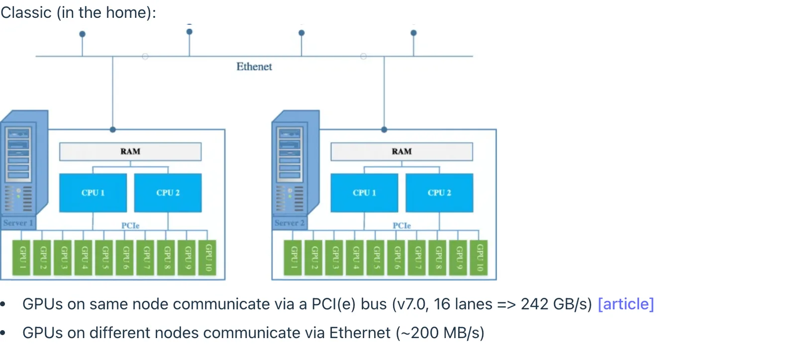
21:53 Okay. So before getting into code, I want to talk a bit about, the hardware, in particular, how GPUs are connected, because we already know what's inside a GPU. so, you know, let's talk about networking, in, in general. So this is kind of a very classic picture. You can tell from this, very old looking image, that, you know, this is how computers used, I mean, generally work. So you have this, you know, server, and then you have a bunch of CPUs. There's a PCIe bus, which you connect things like your, or used to connect things like your mouse and, and, and keyboard. and, and then you have a bunch of GPUs, sitting off of them. And you have some RAM, and then, this computer is connected to Ethernet, to another computer, and so on and so forth.
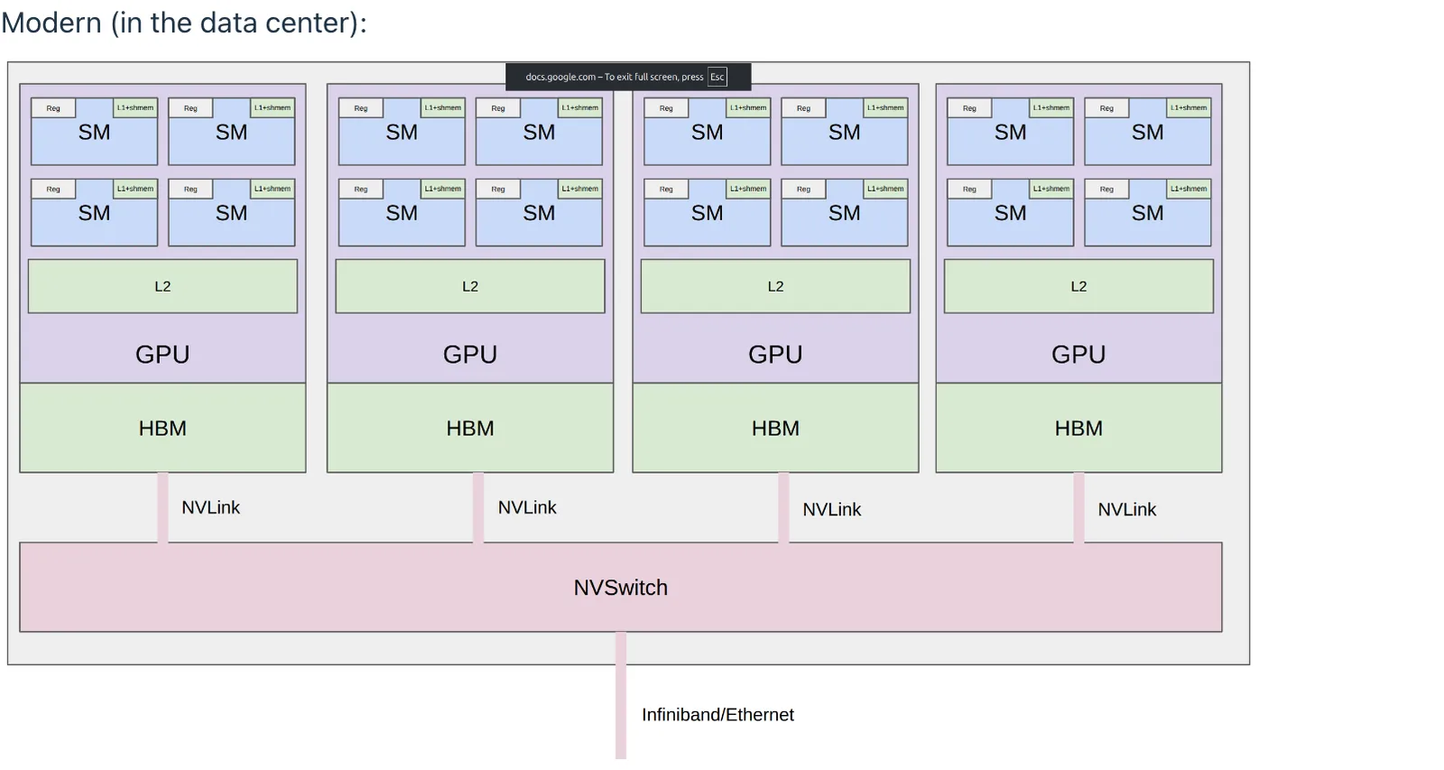
22:46 Okay. So this is a particular setup. It's a particular topology. and, you know, GPUs on the same node, you use PCIe to communicate, and GPUs on different nodes, you have to go all the way through Ethernet. Okay. So this is like if you bought your, like, gaming GPU, and you had, you know, hooked it up with your friend, and it's like, I'm going to train some big model. that's what you would have to do. But, you know, if you're really serious about training, then, things look more like, this. This is the picture I showed in the very, you know, beginning where you have the GPU, and there's something called MVLink and MVSwitch and Infiniband.
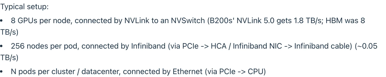
23:30 So, the typical, you know, setup is this. And these numbers, eight is typical, but this 256 is kind of made up. So typically, you have eight GPUs per node. and these are connected via, NVIDIA's MVLink to a switch. and just for kind of calibration, if you use MVLink 5, then you're getting 1.8 terab, it's, terabytes per second. Of total, you know, bandwidth. And remember, HBM was, for B200, was, eight terabytes per second. So it's, you know, about four, about four X, slower.
24:13 So, I mean, this is still pretty fast if you think about, going between devices, but obviously not as fast as, high bandwidth memory, which is much slower than, you know, shared memory or L1 cache. Okay? So basically, a, MVLink connects to the switch. And, which means that, from a programming perspective, you can think about GPUs as connected, to any other GPU. Right? You go GPU to any other GPU, and the hardware takes care of, transmitting that to the switch and the switch routes.
24:51 Okay, so typically, what you will also have is that, at some point, you, you can't have, MV switch and MVLink. And you have to, because one of your clusters, you know, number of GPUs grows, then you're going to have to put these, nodes into pods or, which are connected by InfiniBand. And the way InfiniBand works is that now there's a bit, you know, more, the, so now the, the GPU doesn't connect directly to the other GPU. It has to go through PCI, E, and, and goes through this kind of special InfiniBand cable. And you see that the, the, you know, the speeds are much, much lower.
25:39 And then finally, if you run out of InfiniBand and you have these, like, huge pods, you know, then you need to connect them via, you know, Ethernet. And in Ethernet, you know, you have to go through PCIe and actually goes through this, you know, CPU, which as we'll see is, you know, even, even slower.
26:02 Okay? So it's kind of analogous to the kind of memory situation. The more nodes, you have, then the slower it's going to be. You can't have, like, an Envy switch handling, like, 100,000, you know, GPUs.
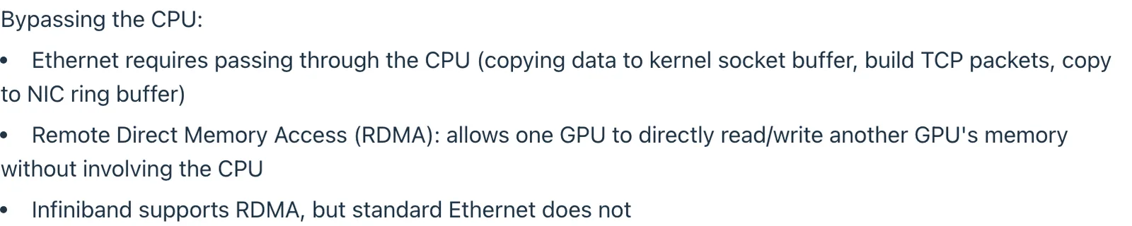
26:18 So one note is that this, I mentioned, alluded to this bypassing the CPU, which is, is going to be, an important thing from a hardware perspective. so if you have traditional Ethernet, you know, what happens is that the GPU has to talk to the CPU to get its, data copied. So it basically has to copy the data, to this, the CPU has a kernel socket buffer. Here is kernel means, you know, not the GPU kernel, but the, the CPU, traditional notion of a kernel. and then it has to build some, some network packets, copy to the network interface, and then ship it over. So this generally introduces a lot of latency. And so there's this technology called remote direct memory access, RDMA, which allows a GPU to directly write or read from another, GPU's memory without using the CPU at all. So, obviously, if you're in MVLink land and MV switch land, then you have RDMA. InfiniBand also supports RDMA.
27:28 So if you're connected via InfiniBand, then you can directly, have GPUs connect to each other without access, involving the CPU. but standard Ethernet, does not.
27:41 there's two notable advancements I will mention is that, so, NVIDIA has been really pushing the limits on what you can do with larger and larger, you know, pods. So they have four of the, basically, the B200s and the, B300s. They have something called MVL72, which means that they, they have these trays of eight GPUs but have nine of them. And so basically, at the end of the day, you have 72 GPUs that are all kind of MV switched into one MVLink domain. And if you remember, the MVLink, you know, speeds are very fast, right? So normally, if you're, if you're, you know, mortal, you think, well, okay, I have eight GPUs that are interlinked really fast. And then outside of that, you know, then things get slowed down a lot. But if you have a lot of money, you can buy this, really fancy hardware. And you can get, really fast interconnects up to 72, GPUs.

28:45 And the other thing I'll mention is that, you know, I said standard Ethernet doesn't support RDMA. But there has been progress on the Ethernet front as well. So there's something called, ROC, RDMA over a converged Ethernet, where the Ethernet actually bypasses the, the CPU. and this is sort of their, their answer to, in, in InfiniBand. So InfiniBand generally is very ex, expensive, as is, you know, a lot of NVIDIA products. but, you can get, you know, pretty good performance by using, using, RDMA over converged Ethernet. And, Meta had some papers showing that they were used, exploring this. So, LAMA may or may not have been trained over, converged Ethernet.
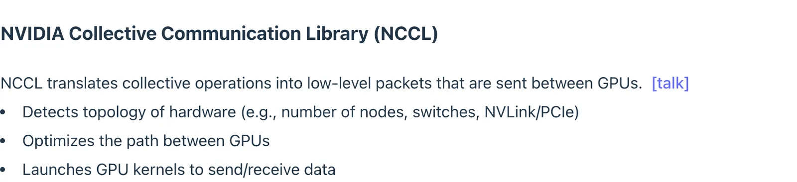
29:42 Okay. So that's just a kind of brief overview of what the, the hardware, looks like. You have GPUs. They're connected via MVLinked to an MVS, switch over some domain, maybe eight, maybe 72. And then it's InfiniBand, from there. And now, let's talk about, you know, how do you program this? So at the very lowest level, there's something called the NVIDIA Collective Communications Library, and, NCCL or Nickel, which translates the collective operations, the all reduce, reduce broadcast, into the actual low-level packets that are sent between GPUs. So what a Nickel does is it, when you, when you use Nickel, it's basically like saying, I want to all reduce. And then Nickel goes and figures out what is the topology of the hardware, figures out the, the path between different GPUs, and then it actually launches the GPU kernels to send and receive data.
30:43 Because at the end of the day, remember everything that runs on a GPU is, is a kernel. So there are communication kernels as well that actually do, you know, communication with other GPUs. Okay, so we're not going to look too, too much more into, Nickel, but just know that it exists. and then we're going to actually go to PyTorch. So maybe before that, any questions about, you know, hardware?
31:12 Yeah? Can you, like, describe physically a rack and a tray?
31:20 can I describe physically a rack and a tray, like what a rack is and what a tray is? so for the MV72, so I'm not, I'm not a hardware expert, but, but a rack, I mean, is literally like, I mean, I've, I've seen data centers, like literally a, a rack. And each tray is, something that has, so, so G, the G stands for a great. So there's, you know, two CPUs and each CPU is connected to four GPUs. So each tray has, eight, GPUs on it and they're stacked and everything, you know, is connected to this, you know, MV switch.
32:06 Yeah?
32:11 Yeah.
32:15 Yeah, so the question is what is the difference between RDMA and the. Yeah, so RDMA, you can think about it as a more of a, a desiderata. RDMA means that, like, one GPU can read and write from another GPU's memory. And there's multiple ways to do RDMA. One is to use MVLink and MV switch. And another way is to use InfiniBand.
32:45 So, the, the, the, the, the, the, the, the, the, the, the, the, the, the, the, the, the, the, the, the, the, the, the, the, the, the, the, the, the, the, the, the, the, the, the, the, the, the, the, the, the, the, the, the, the, the, the, the, the, the, the, the, the, the, the, the, the, the, the, the, the, the, the, the, the, the, the, the, the, the, the, the, the, the, the, the, the, the, the, the, the, the, the, the, the, the, the, the, the, the, the, the, the, the, the, the, the, the, the, the, the, the, the, the, the, the, the, the, the, the the, the, the, the, the, the, the, the, the, the, the, the, the, the, the, the, the, the, the, the, the, the, the, the, the, the, the, the, the, the, the, the, the, the, the, the, the, the, the, the, the, the, the, the, the, the, the, the, the, the, the, the, the, the, the, the, the, the, the, the, the, the, the, the, the, the, the, the, the, the, the, the, the, the, the, the, the, the, the, the, the, the, the, the, the, the, the, the, the, the, the, the, the, the, the, the, the, the, the, the, the, the, the, the, the, the, the, the, the, the, the the, the, the, the, the, the, the, the, the, the, the, the, the, the, the, the, the, the, the, the, the, the, the, the, the, the, the, the, the, the, the, the, the, the, the, the, the, the, the, the, the, the, the, the, the, the, the, the, the, the, the, the, the, the, the, the, the, the, the, the, the, the, the, the, the, the, the, the, the, the, the, the, the, the, the, the, the, the, the, the, the, the, the, the, the, the, the, the, the, the, the, the, the, the, the, the, the, the, the, the, the, the, the, the, the, the, the, the, the, the, the
34:13 the, the, the, the, the, the, the, the, the, the, the, the, the, the, the, the, the, the, the, the, the, the, the, the, the, the, the, the, the, the, the, the, the, the, the, the, the, the, the, the, the, the, the, the, the, the, the, the, the, the, the, the, the, the, the, the, the, the, the, the, the, the, the, the, the, the, the, the, the, the, the, the, the, the, the, the, the, the, the, the, the, the, the, the, the, the, the, the, the, the, the, the, the, the, the, the, the, the, the, the, the, the, the, the, the, the, the, the, the, the, the
34:44 So the question is what happens if you have nine GPUs? How do you distribute the workload across those?
34:53 I suppose, I guess it kind of depends on how the nine lands in your, your setup. For example, a lot of times you'll have, you know, let's say you have eight GPUs per node. So then the ninth one would be on a different node and if you don't have, you know, MVs, link connecting them, then that's going to be really bad because that's going to be one node which is not providing that much compute and also very expensive to communicate with. but if you, let's say, had, everything were connected by MVs, you know, switch, then it would be, much more reasonable. Okay. one more question and I'm going to move on. Yeah. How is this different from TPUs? So how is this different from, TPUs?
35:42 so Tatsu described TPUs a bit, more. So, I mean, the, let's see. what can I say quickly about this? so TPUs are generally kind of much, you know, simpler objects. I'm not too familiar with the details of how this, like, what this, each of these components corresponds to,
04 torch.distributed 编程与演示
36:09 but maybe we can talk about it often.

36:13 Okay. So let's actually get down to some code to, take advantage of this, this hardware. So PyTorch conveniently has, Torch.distributed library that provides a clean interface into these collective operations. so you don't have to explicitly think about Nickel. and in fact, this library also supports different backends for different hardware. So if you are on GPUs, then you would use the Nickel backend. And if you're on CPUs, then there's something called Glue, which, still allows you to, you know, like I said, parallel processing has been around for, you know, a long time before GPUs. And you can do, these collect operations on CPUs as well.

36:59 this library also supports higher level models and algorithms such as, FFTP, but we're not going to use those in the course because we're building things from scratch. All right. So let's walk through some basic examples of collective operations. so there's, this function called, spawn, which takes, another function I'm going to call. And it says, I'm going to run this, replicated four times where four is the world size. So let's see what this does. this is actually a wrapper I wrote. just to sort of hack around the fact that I can't do multi-processing in this, this lecture. So normally what you would do is you call, you know, torches multiprocessing.spon and you call the function.
37:54 but, you know, I'm going to do this branch which disables distributed. So let's just go through that. So now, now I'm in this, function that it's supposed to be running on asynchronously for each process. So remember world size is a number of processes. And the rank is either zero or one or two all the way up to world size minus one. And so there are world size number of these functions that are each running on a process at the same time. Okay. So I'm on rank zero right now. So what do I do?
38:32 there's a setup. you basically configure, the, the master address and port. notice that this is not actually how the, the GPs are going to communicate. This is more for just general metadata and coordination. The actual data goes through nickel. Otherwise, it'll be very, very slow. and if you have CUDA available, then you can use the nickel backend. I am on my laptop, so I'm going to use, the glue backend. Okay.
39:04 So, so now I'm here, I'm running, you know, pretend I have four of these processes running. so there's this, barrier function, which, is useful as, it's a synchronization barrier. So basically, if I see this, then it waits for all the processes to get to this point. okay. So, basically, you can think about all the processes are running asynchronously. so I don't really control one could completely finish before the other. They might, finish, be interleaved in any way. So if I want to make sure that certain, there's some code that is executed before other code, I put these, synchronization barriers in. So now the downside of putting more barriers in is that, well, you end up kind of waiting, potentially unnecessarily.
40:00 Okay. So let's try an all reduce. Okay. So I'm going to, create this tensor, 0, 1, 2, 3. And, I have my rank just to make it more interesting. Each rank is, going to have a different tensor. I'm gonna print out what I have before the all reduce. So now I'm gonna skip over here and see what gets printed out. so, rank 0 before all reduce has 0, 1, 2, 3.
40:35 rank 1 has 1, 2, 3, 4, and so on. It's the same example as I showed before. Notice that the print statements are coming in whatever order, the hardware feels like it because it's running async. But all the data is there. Okay. So now if I do an all reduce and, this, you pass in, this is a PyTorch function. It passes in this, this tensor. You pass in the reduction operation, which is a sum. And I'm going to say don't do, async.
41:08 And what this does is it calls, in this case it would be glue, but it could be nickel. And which, in which case it would spin up the, the CUDA kernels. It would do the communication. It takes here everything for you. And then it basically writes in place to the data. So after the all reduce, I have the all reduce operation. Remember, which is the sum of each of these columns, but replicated across all the ranks.
41:40 Okay. So, so that's, you know, all reduce. And if you wanted to be, you know, fancier and do async, then you could say async equals true. But then it would screw up all these print statements. So I'm, trying to put more barriers than I would normally would.
41:58 Yeah. Question. In this case, the rank is the, other, person.
42:07 so the question is the rank to GPU. for this class, the rank is, the GPU. Yes.
42:18 Okay. So let's try another example here. so I'm gonna do a reduce scatter. So here, I'm going to create an input, which is zero through the, the world size. and, I'm going to, have, the, the output. I'm gonna allocate the output. And so what does this look like before I do the reduce scatter? It looks like, let's see, this. Where each, it's a, kind of the same, you know, input.
42:59 And the output is, happens to be zeros. But it could be, you know, just anything. And then, I do the reduce scatter tensor. Here, instead of writing in place, I have a, output tensor and an input tensor. I say I wanna, you know, do the sum. And then afterwards, I get, basically the input is not touched, but the output, I get the, the reduction of each component written into the respective, ranks.
43:36 Okay. So, yeah, question.
43:41 .
43:50 Yeah, so the question is, how does it work to do the all reduces asynchronous? So, what this means is that this, this is sort of like a monolithic operation. You say, go do the all reduce. And it's spinning up, you know, CUDA kernels. It's going to, you know, do the communication. And, remember CUDA is already kind of async, with respect to the process, the processes. And now we have all the processes being async. And the point is that, this code just would return. and, and then you could do kind of other things.
44:29 So, a typical thing, which I'm not gonna have, talk about this class, is overlapping computation and communication. so, for example, you can do this, operation. And then you can go ahead and load some other data for the next, step. which is independent of this operation. And then when you wanna make sure that you actually, are done, then you can call a wait or a, a barrier.
45:02 Okay. So, let's do the final one, which is all gather. So, by now, I think you kind of get the idea. Here, I'm going to set as the input, the output of the reduce scatter. I'm gonna allocate an output. so before the all gather, it looks like this. I have my results from the reduce scatter here. the output is, you know, it just allocated. It happens to have some values in it, but don't, you know, worry, about it.
45:36 and then, after I do the all gather into tensor, and then I will have, you know, all the different, inputs, you know, gathered onto all the different ranks. Okay. And you can see here that indeed, proof via example that all reduce is equal to reduce scatter plus all gather.
46:13 Okay. And then, just to wrap things up, just as I started by a setup, then I clean up, which, you know, just, it's good practice to clean up.
46:29 Okay. So, so that was your first example of a Torch, distributed, you know, program.
46:37 Okay.
05 基准测试:实测 NCCL 带宽

46:38 So let's do, some, you know, benchmarking. this will be quick since I want to actually move on to the, part two. so how fast does communication happen? So let's do an all reduce. so here I'm going to all reduce with, you know, 100 million, elements. And, oops.
47:08 Okay. Let me, sorry, mess this up.
47:14 Okay. So I'll reduce. So I'm going to create, you know, this, this sensor with this number of elements. Call, and remember just like before when we do benchmarking, we warm up first. and here I'm going to call the CUDA synchronized and also the, the barrier, just to make sure that, because there's two forms of asynchronous here, the CUDA kernels and the different processes. And just want to make sure everything is kind of, not running and, is, is done, before I start the time. And I'm going to do the all reduce, and, and then wait, again with the synchronizing the barrier and stop the time. Okay. So, remember this is running for every single rank.
48:08 So if I look at the output here for rank 0, 2, 1, 3, I have a different time potentially because they're all different processes. each of them is going to report a certain, you know, measurement. And if you want to report one number, you can take the average for example. so now one thing, that is, useful to do, which is analogous to when we were computing MFU, is to compute, measure the effective bandwidth. And the idea here is that, well, this took 1.6 milliseconds. You know, how much, you know, is that good or bad? So to compute the effective bandwidth, what we're going to do is to compute essentially how much, how many bytes were sent and should be sent kind of during this computation. and then you divide by the total time, then you get the bad, effective bandwidth.
49:09 Okay, so, the size of what I'm sending around is the, the size of each element times the number of elements. So that's the basically the number of bytes of this data tensor. how many bytes get actually sent? So this, needs some unpacking. So for all reduce, if you think about, let's just say for simplicity, you do a rank 0 plus rank 1 plus rank 2 plus rank 3, you need to iterate this world size minus 1 steps because there's a world size minus 1, you know, addition operations though. So that's this factor. There's a 2 because you need to both kind of send and reduce. So, and then you multiply by the size of the payload. So that's the total number of sent bytes.
50:02 And the total duration, is the, the time that the wall clock time that it took. And then you multiply by the, the world size, because it's like the total amount that the, all the ranks have weighted. And the bandwidth is the, the, the byte sent divided by the total, you know, duration. Okay? So in this case, you get something like, you know, about 400 gigabytes, you know, per second.
50:41 Okay? So one, a few notes here. One is that the effective bandwidth, if you look at this expression, size times 2 times world size minus 1 divided by world size times duration. So as world size increases, this, world size minus 1 divided by world size essentially converges to 1. So you're effectively left with 2 times the size bytes over the duration. So this is essentially, the bandwidth. Notice that this is independent of the world size, which is, which is good. So if you grow the number of GPUs you have, you are still, you know, the bandwidth doesn't, you know, change. It is also independent of the topology, which is something that kind of nickel, you know, figures out whether you're, going to, pass the messages in a kind of a ring or a tree topology.
51:31 so, yeah. Okay. So that is, all reduce. And for reduce scatter, this is very similar. so I'm going to create the inputs and the outputs, warm up, perform the operation, and time it. So, notice that the reduce scatter has, this, these timings. and, and you can also measure the effective bandwidth here. The number of bytes, that were, in the input, you have the number of bytes that were sent. Here there is no, you know, 2x here.
52:19 and then the total duration, you divide by that, you get the bandwidth. So here, the bandwidth is, it should be very similar. I guess sometimes there's some stochasticity, but it's on, in the kind of 400s.

52:36 So a few notes here. All reduce is, remember, as we stated, reduce scatter plus an all gather. And so all reduce naturally is moving twice the amount of data, because reduced scatter is, like, has some costs. All gather has some cost. And all reduce is doing twice as much work. but, and it takes twice the amount of time. but, you know, the two cancel out, so you get the, the same kind of bandwidth.
53:17 Okay. All right. So, that is the end of part one. Maybe, any questions before I move to part two?
53:29 Yeah. Why do you do that synchronize for the Cuda kernel?
53:40 So why do we have to do the synchronize for the Cuda kernel? So, at the end of the day, we are still doing Cuda operations. Right? We have just multiple processes, each with a GPU, doing some Cuda operations. And then, so if you're doing a Cuda operation, remember, by default it's async. So when you reach the next line in Python, that Cuda operation might not be done. So we need to wait always until that's, to make sure it's done by synchronizing. Yeah. So, would you have to first do barrier and then synchronize?
54:17 So do you have to do barrier first and then synchronize? not sure. Yeah. I would think if you want to use the first set all divided into the code and then wait for all these. Yeah?. Yeah. I think one problem is if you barrier first and then the Cuda might not be done running and you just immediately go to the barrier and then you are still kind of each independently synchronizing the different Cuda kernels, which means that you're not really synchronized on, like the barrier might, if all those operations just return, the barrier doesn't really do any.
55:06 Okay.
06 数据并行(DDP):按 batch 维切分
55:06 Okay. Let me move on. So now let's actually start thinking about how you train models. Okay? So we're just going to walk through a very bare bones implementation of training MLPs, multi-layer MLPs. I guess that's redundant. It's multi-layer perceptrons already. and remember that MLPs are the ones that are the actual compute bottleneck and a transformer. So this is actually pretty representative of what you'll see.
55:33 Okay. So data, parallelism, tensor parallelism, and pipeline parallelism. And the picture I want to, what you to have in your head is this picture. So, this is a little bit of a semi-schematic, so don't think too deeply about this. But it's more of a way to conceptualize how you're cutting, your data and parameters. So data parallelism says I'm going to split the data into pieces, and then each of the GPUs is going to be responsible for part of the data. And I'm going to do normal, you know, I'm going to keep track of all the parameters and do model, normal model, you know, training. and then I need to synchronize. So let me explain how this, how this works.
56:24 So I'm going to generate some sample data. So there's a batch size of 128, number of dimensions 1024. So this is a batch size by numdim, matrix, data matrix. And, let's jump into this, data parallelism. Okay? So the way that it's going to work is that you have this data matrix, and I'm going to break up the rows into a bunch of, into num- world-size pieces, and this case four, and each, rank is going to get a piece. Okay? So the number of dimensions, the batch size, so each, I'm going to call the local batch size, basically, you know, the batch size divided by the world size, which is every row is going to, that, GPU sees is going to have 32, you know, data points. and this is just indexing start index, data start to end gets you the slice of that data.
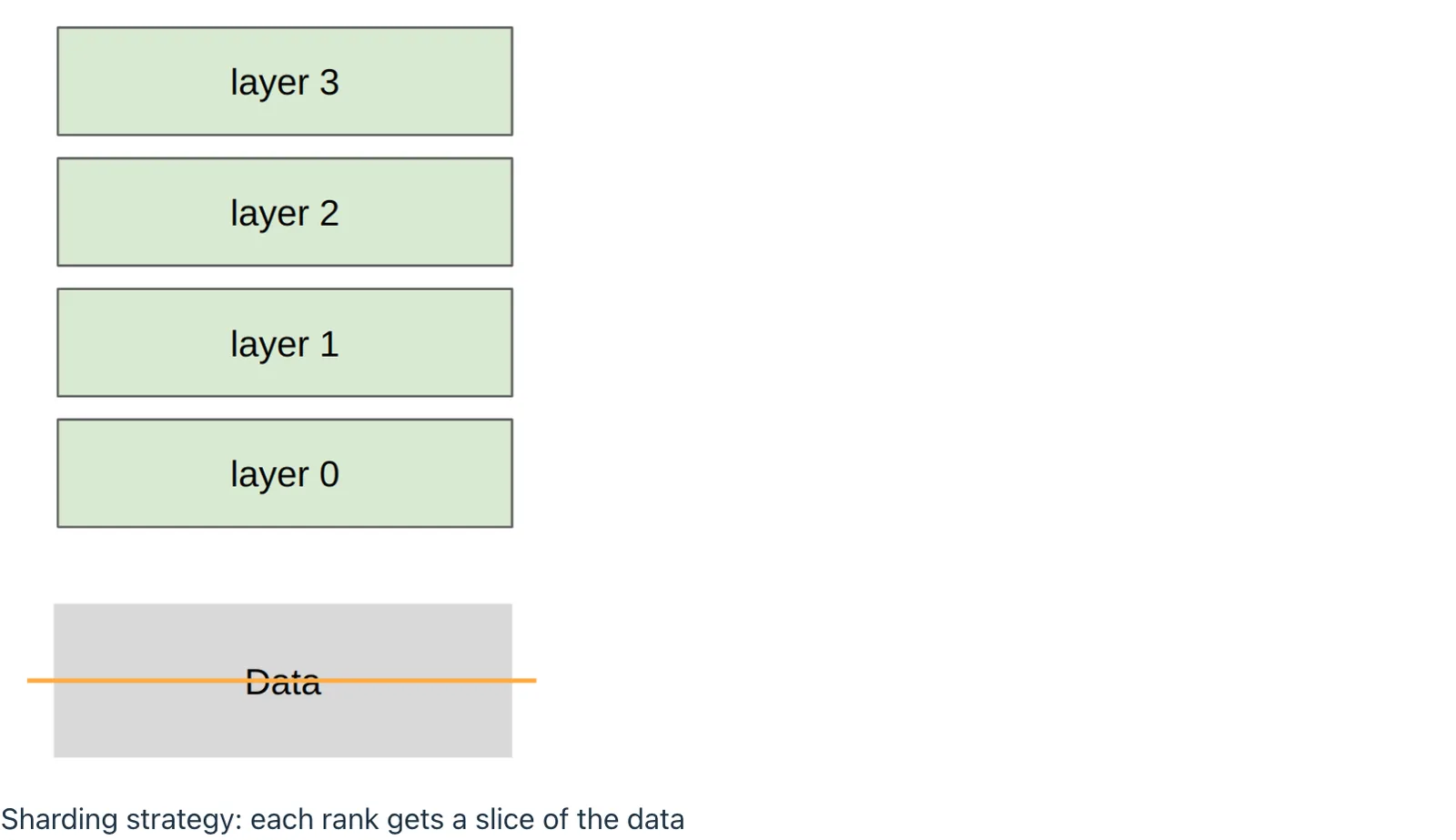
57:37 And I'm going to just put it on that, on that rank. Okay? So at this point, each GPU has now a distinct data tensor, which is the part that they're responsible for. Now, in practice, each rank should probably load its own data, rather have this, you know, this bottleneck, but, this is just for illustrative purposes.
58:04 Okay. So let's, instantiate the, the MLP. So here, I'm, assume we have num layers, and, num layers, and for each of the layers, I'm going to have just a num dim by num dim, matrix. so I'm just going to initialize a random, you know, set of parameters. and then, I'm going to feed that into optimizer. Okay? So here's the training loop. So in the forward pass, I take the data. So remember, data is not all the data.
58:45 It's just, if I'm rank two, then I only get B two, part of the data. I'm going to just, you know, go through the number of layers and, do a forward pass. And then I'm gonna do a backward pass. And then normally, this would be it. But, now remember, every rank has different data. Therefore, the gradients are going to be, you know, different as well. So this is the key, step that makes, data parallelism work. We're going to synchronize the gradients across all the workers. This is the only difference between standard training and DDP.
59:24 It's actually pretty nice and elegant. So basically for all the parameters, I'm going to do an all reduce of, pram.grad. And I'm going to average, and then after this all reduce is done, then now at this point, each of the ranks has the exact same gradients.
59:52 And then I'm just going to update, the, the parameters.
59:59 Okay? So it's kind of really kind of elegant, I find, because it's basically standard training, where you apply it to your local batch. But, you just insert this after the backward pass. Let's just, you know, average all the gradients via this all reduce. It's a one line, you know, code change. And then the parameters get updated. So as you're training, each, rank is basically performing parameter updates as if it were, have all the data on it. But it's only actually processing a part of the data.
1:00:35 Okay. So that's basically, DDP or, the, first type of data parallel.
1:00:43 Any questions about this?
1:00:46 Yeah?
1:00:51 So the question is, can you only do this with batch size greater than one? yes. So your batch size has to be at least world size for this to really make sense. And usually it should probably be quite a bit larger.
1:01:08 Yeah?
1:01:10 Yeah. Yeah. So the question is, should the, batch size be a multiple world size? And that's also would be nice. Yes. I mean, if it's not, then you can pad it with zeros or something. So there's ways, but it's just easier for everyone if it is. Can you talk about, DDP for a transformer?
1:01:42 yeah. So the question is, what would this look like for a transformer? It would actually be basically, the same. The DDP has a nice thing that is very modular. You do the forward pass. Look, I mean, DDP just averages the parameters here. It doesn't care what your forward pass looks like.

1:02:04 Okay. Let me move on. Okay. So that's DDP. so just to summarize, the losses are different across the ranks. the gradients are also, you know, initially different. But they are all reduced to be the same across the ranks. And therefore, the parameters all remain the same across ranks. Okay.

1:02:32 So next lecture, Tatsu is going to talk about fancier, data parallelism, FSTP and zero. And the idea there is, as I've alluded to, here we use all reduce. It's like a very simple monolithic operation. But it does require holding all the map models parameters in memory. But what if the model parameters don't fit in memory?
07 张量并行:按宽度维切分
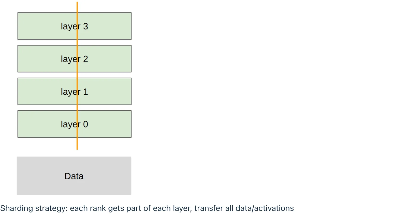
1:02:53 Then you're going to have to be more clever and that's the topic for next class. Okay. So let me talk about tensor parallelism. so here the idea is we're going to cut this way. I mean, we're not going to cut the data. We're going to cut, the, essentially, each layer. And so each rank is going to get part of each layer. Okay. And generally this rem- means that we're going to have to transfer a lot more, more data.
1:03:29 We're going to discuss this a bit later. so what does tensor parallel look like? Okay. So, we're just going to assume we have this data. Every rank has all the data, just for simplicity. And here, remember the, the data is batch size times num dim. And I'm going to define a local num dim to be for this, rank. I only am, responsible for a subset of the dimensions. So, the, kind of the picture here is that, each model still has all the layers here, for all the layers.
1:04:16 But the parameters now are num dim times, local num dim.
1:04:23 Okay. So if this were one of the parameter matrices for one layer, I would be doing, splitting down, the columns. Okay. So this is also known as column, you know, tensor parallel. You can also do it by rows, but we're not going to talk about that right now. Okay. So now what does a forward pass, look like? So go through all the layers and I'm going to compute activations.
1:04:53 So, I start with, you know, x, the data. And I'm going to access the parameters at layer, layer. And notice that this is only a slice of the parameters, right? So if I'm on rank one, I only get this part of, the matrix. But, you know, I can still proceed. I can apply this non-linearity because this is element wise anyway. but now what I'm going to do is I'm going to, you know, communicate activations. So if I have a data matrix, rank one has activations for part of the activations, for this part of the matrix, rank one has part of activations for this matrix and so on and so forth. And I need to basically put all the activations on all the, the ranks.
1:05:52 And, but we know how to do that. We introduced all gather as a collective affirmative. So I have, this is all the, the activations. so this is, you know, the batch size times local num dim, which is the shape of the, of the activations. and then I'm doing an all gather. sorry. So this is the allocating memory for the activations. So X is the actual part of the activations. So this is batch size times local num dim.
1:06:30 And all gather says each rank has X and each, rank is all, are going to allocate activations, which is a list, one for each world size. And then after the all gather, X is going to be copied into each of the respective location activations.
1:06:53 Okay. So then, once I gather all the activations, I concatenate them to form the full, dimensional X, which is batch size times num dim.
1:07:08 Okay. any questions about column tensor parallel?
1:07:17 So this is done for every layer. we've now noticed one difference between, data parallel is now we have to kind of muck around with a model. Data parallel is very elegant because it's splitting by data. The model is treated as a, as a module. but now we have to muck around with a model. and, you know, this is sort of strongly leveraging the fact that if you want to do a matrix multiplication, you can split it up into a set of small matrix, small, small matrix multiplications, we can do those on different ranks, and then we can gather the, the results.
1:07:58 .
1:08:04 Yeah.
1:08:07 So, so now the question is what happens in backprop. Now, in the backprop, you have your, your activations, and you have to, reduce, scatter to all the different, you know, gradients. So in some ways, all gather and reduce scatter have this kind of duality where in forward, if you're all gathering in, in the backward, you're reduce scattering.
1:08:33 Yeah. So the question is, is that done automatically by autograd? So none of this, w- okay. So if you just call dot backward, it's not gonna do it because there's no parallelism in that. But, you know, PyTorch has all these things that are done automatically for you. So,
1:08:58 .
1:09:09 So in this, so what is done for you versus automatically, here we're managing things fairly explicitly. So, which means I'm not doing the, backward pass, but you would have to manage and call the, the reduced scatter yourself. Yeah. Yeah. And that's by design because this is 336, you know, building language models from scratch.
08 流水线并行:按深度维切分与微批次
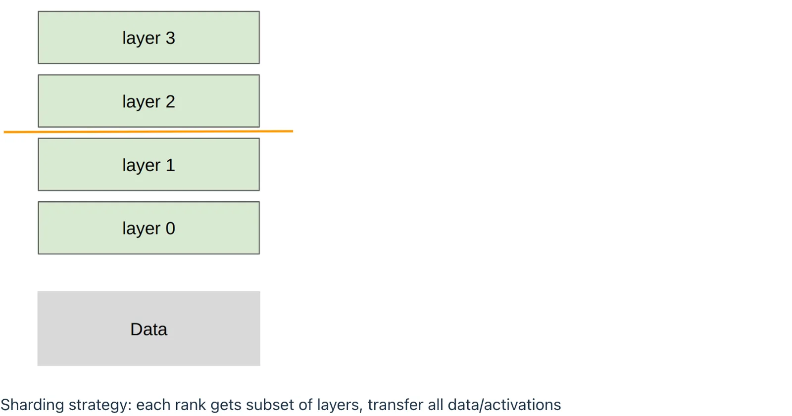
1:09:35 In practice, you probably wouldn't have to do that. Okay. So let's do pipeline parallelism, quickly. So the idea behind pipeline parallelism is we're gonna split the network this way. So each, rank is gonna get a subset of the layers now. Within each layer, it's gonna get all the, the dimensions. And it's also gonna get all the, well, the, one of the ranks is gonna get all the data. it's gonna, every rank is gonna see all the data in some form. so this is the, the way it's gonna work.
1:10:12 okay. So let's, we have all the data, which is again, the batch size times numdim. and I'm going to split up the layers. So local num layers is going to be the number of layers that a particular rank is going to handle. and, and so now I'm gonna have local params, which is basically only there's local number of layers, number of them. But within each layer, I'm going to do the, you know, numdim by numdim. Okay, so, one thing I, maybe Tatsu will talk more about this on, Wednesday, is this idea of micro batches. so maybe I'll just present this and explain why I'm doing things this way. So in addition to splitting up the layers, I'm also going to split up the batch into a bunch of micro batches.
1:11:13 so if I'm rank zero, then I get the data. and I'm gonna chunk it up into a number of micro batches. and for each, you know, micro batch, what I'm going to do is, receive it from the previous rank. and then do the feed forward pass only on the layers that are assigned to this rank. And then I'm going to send to the next, you know, rank. Okay, so here I'm actually using these receive and send, which are point-wise operations. I, so I didn't cover those before, but they're fairly, explanatory. This basically says I'm rank and I'm going to send this tensor over to, you know, sorry, I'm gonna receive this tensor from rank minus one. and this says I'm gonna send tensor X to rank plus one.
1:12:19 okay.
1:12:27 So, so basically the reason why, I'm talking about micro batches is, and Tatsu will talk more about this, on Wednesday, is that in pipeline parallelism, so you have one rank that gets the data, it processes some of the layers, and then it sends it to the next, you know, GPU, and it processes some of the layers, and it then sends it to the next GPU. Right? So this is a very natural way of dividing out a deep network, but the problem is that you get these, what we call pipeline bubbles, where, while you're not, sort of processing, you're kind of waiting around for other tensors to process. And this is, ends up being quite inefficient. So the idea behind, micro batches is that you break it up into smaller batches so you can kind of process it quickly, send it on to the next one, so this can reduce the number of, pipeline, you know, bubbles.
1:13:32 Okay. So the other thing I will mention that is not handled in this very kind of naive version is the idea of overlapping communication and computation, which is actually very important to pipeline parallelism. This basically gives you the right structure. If you put an I, before these, then it becomes, kind of async. you, you have to add more things to kind of manage the, the, the code. and the idea here is that you want to be, while you're computing here, you should, you know, you can be receiving, data or sending data. So computation and communication should be overlapped so, that reduces amount of time, you're actually spent waiting.
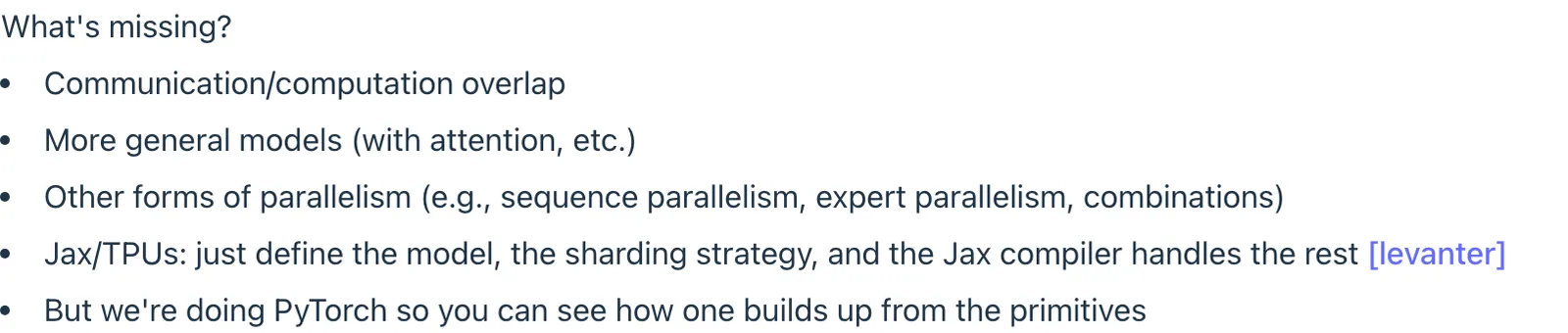
1:14:22 Okay. So a few things are kind of, you know, missing here, which we'll, hopefully fill in next time. So the communication versus computation overlap, which is, especially crucial in pipeline parallelism. I didn't mention, in data parallelism, this also, happens because I just did a forward pass and then at the end I'm just doing all these all reduces. But if you're clever, then on the backward pass, as soon as the gradients are done, you can start sending that. And that's something you're being explored in the assignment two. And this again allows you to just, you know, overlap communication and computation, more. we had some questions about what about general models. Again, I think this, MLP gives you essentially all you, you know, mostly of, most of kind of what you need for understanding the, you know, the basics.
1:15:27 some of the larger models just require a lot more bookkeeping. So, it's harder to kind of see the core, core algorithms. there are other types of parallelism that we haven't covered. so sequence parallelism takes a whole, you know, sequence and chops it up into pieces. And that allows you to parallelize attention computation. Expert parallelism, which, allows you to parallelize, the experts for MOEs. And this is where the all-to-all that I mentioned comes in. And then also, you know, you know, different combinations of, different parallelism techniques, which also will show up in the assignment. so one thing to note is that the, which parallelism technique you choose is going to be strongly dependent on the hardware.
1:16:21 For example, tensor parallelism, there's a lot of communication because for every layer you're just, you know, you need to send all these activations which are fairly big. So generally, tensor parallelism happens within a node on MVLink or MV, where you have high bandwidth. whereas you wouldn't do tensor parallelism past the kind of MVLink, you know, domain. whereas a pipeline parallelism, you'll see people using it. And generally, this is, can tolerate much, you know, slower, you know, interconnects. So some of the, the centralized, training work uses pipeline parallel because your, you know, nodes are, GPUs are actually across, halfway across the world. but you wouldn't want to do tensor parallel in that, that setting. so sometimes you, when you look at these combinations, it will be tensor parallel within node. And then, and then, you know, pipe data parallel or FSDP.
1:17:28 And then, and then, you know, pipeline parallelism if you, if you need it. there's other effects such as if you do data parallel, you might be able to do data parallel, quite a bit. But then, you start heading to something called the critical batch fact, size where if you start increasing the batch size too much, it doesn't actually help you. In which case, you're just kind of wasting your compute and then you're better off using tensor parallel. So there's a bunch of these considerations which, we'll talk more about as we, go through the class. so final note, so TPUs kind of came up a little bit. one thing to, to note is that on purpose we are using PyTorch and not just using PyTorch, but really using the collective, operations in a very primitive way. So you can see, mechanically what's happening. Another approach, especially if you're in your Jackson TPU land, is that you can simply define the model and the sharding strategy.
1:18:35 And the compiler actually handles a lot of, the, the decision of how to, basically, what kind of communicating operations you need. You basically say, well, this piece of data needs to be here and here and here, and then the compiler does, some magic to figure out what. so that's appealing, but, you know, obviously it would take a lot of the, you know,
09 总结与展望
1:19:03 the joy out of actually building things from scratch. Okay. just to summarize. So there's many ways to parallelize. you can cut by data, cut by tensor or, expert, cut by pipeline or sequence. we looked at data parallelism. we only did DDP. Next time we'll do FSTP and, zero. tensor parallelism, as I mentioned, requires very fast interconnects.
1:19:36 Pipeline, less so. but you need to really work hard to reduce these pipeline, you know, bubbles. and then maybe at a high level, we see this kind of, you know, pattern come up a lot. Right? So you can either recompute or store in memory. when we were talking about things like activation checkpointing or, doing, you know, when we're working with GPUs. Or in this case, you can think about an extension of this is that you can store, on a different, you know, GPU. Right? From that perspective, you look at the data parallel.
1:20:14 Right? You're doing redundant work in some sense because every, you know, rank is actually updating its parameters and keeping track of all the parameters. But the reason you're doing that is that you don't have to move the optimizer state across. so, you know, one thing is that, you know, hardware is getting, you know, faster. But in some sense, we'll always want, you know, bigger models. So this idea of having a hierarchical structure will, you know, always be there. Okay. So that's it for today. So, next Wednesday, Tatsu will, do more of a deep dive on, more parallelism techniques.
1:20:56 Okay.