缩放定律：案例与实践细节

01 开场：为什么要关心 scaling 的实践细节

0:05 OK, we're going to continue our scaling journey. Today is a bit of a grab bag of stuff. I mean we're really going to talk about some of the more advanced details of scaling laws, and how we scale up models. And in doing so, we're gonna cover what I feel like are some important details in how you know you would scale up a language model in practice. OK. So, you know, we might want to ask some questions. You, like, is the scaling lost stuff that you talked about two lectures ago, you know, does that actually work at real building open source model scales? It would be nice if we could optimize some of this. There's a lot of like learning great tricks and other things that people do, that I think you should know as people that are informed about how to build a language model. #

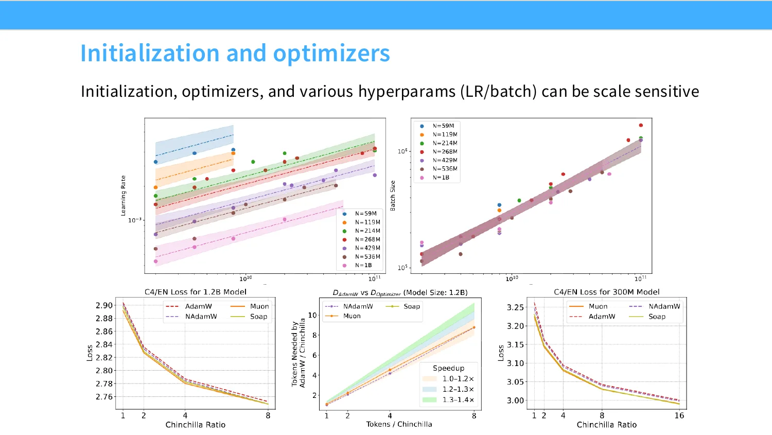
0:51 So we'll talk about some of these optimization details. And then I think the last thing I wanna talk about is when we scale up, there are certain things that are going to be a little bit trickier to tune. We know that optimizers and optimizer behavior is going to be actually pretty scale sensitive. and because of that, things like initializations, learning rates, batch size, those we need to carefully think about as a function of scale. so we will talk about How to think about those carefully. #

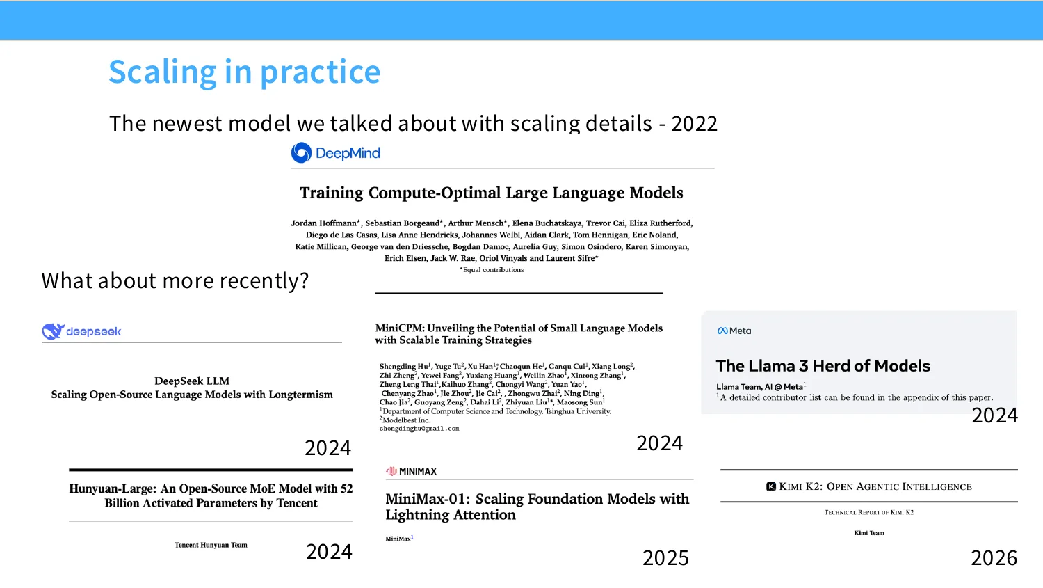
1:20 So up until now, most of our discussions what I would is what I would call like the classical, you know, scaling laws canon. We talked about Kaplan, we talked about Oh, even Hestness. And then, you know, the transformer paper, right? So so we're up to date with I don't know 2022 or something. Since then, you know, there have been a number of scaling papers that are published by people who train big models. Although I think the number of such papers have decreased in recent years, and most of them have come out of the open source community in China. And so today, I wanna talk about a number of these that I've sort of curated and selected. To give you a sense of, you know, what does scaling at the frontier, at least open frontier look like? What are the things that these people care about or worry about? #

2:05 And like, what would what would you need to do? to sort of speed run your way from Kinkajou all the way to, let's say, Kimmy K two. Most recent release that has some scaling details. OK, so that's gonna be the first part of this lecture. We're gonna go through a couple papers, and we're gonna go through the details. The second part is going to be a discussion of optimizers and initializations. And remember I spent a non-trivial amount of time two lectures ago on the selection of batch sizes. That's gonna be an important factor, and it's also gonna be important thinking about how we're gonna tune things like learning rates. Those are very sensitive, very important to get right. #

2:41 And so it turns out that a lot of effort has been invested into getting those things right, and we will talk about Some of the techniques to do so, and this may in fact even be useful in your day to day lives of training various language models. because they'll give you a sense of how to change your hyperparameters in your experiments as you scale up or down. #

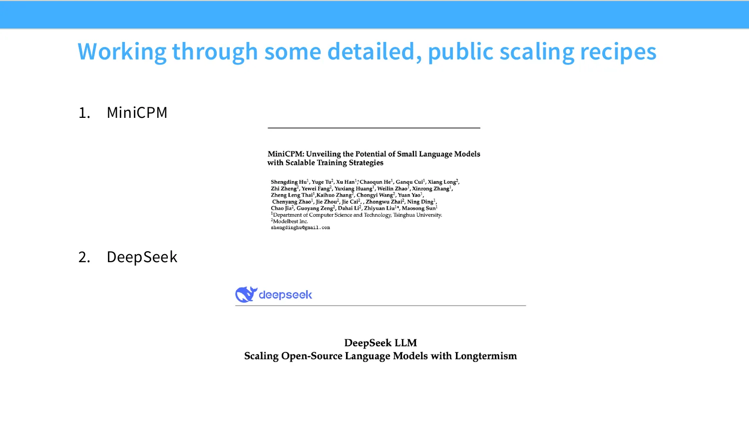
2:59 So, I'm gonna spend a non-trivial amount of time talking about two papers in particular. They're not the newest papers. They're not necessarily the most Actually, deepseek one might be one of the more detailed ones. Most detailed scaling paper in general, but I think this is s- hits a sweet spot. So both of these papers are kind of serious Scaling investigations from people who build, you know, reasonably high performance models. And importantly, they take pretty different approaches to some of the key questions that we will ask today. #

02 MiniCPM：muP、最优 LR/batch 与 WSD 学习率

3:30 And so I think they're a good way to motivate a lot of the rest of the lecture. So I'm gonna talk about these two. First one's Mini CPM. This was I think back in 2024, high performance small language model. In deepseek, you all are now familiar with this, I no longer have to justify why I'm talking about deepseek, which is great. We'll start by talking about mini CPM though. I I do like this paper, especially when it first came out, it felt very fresh and new, and like very, you know, at the cutting edge. Even in 2026, I feel like a lot of the things that the mini CPM folks did is very informative to us. I'll talk about this later as I get to the newer papers, but I think it's kind of becoming the case that a lot of this like Classic scaling stuff, like how you set learning rates, how do you do Chinchilla? #

4:14 Those kinds of things, I think are now taken for granted, like everyone just assumes that you know how to do those things. And so people don't really talk about those as much anymore in the paper. So it's really nice to talk aboutum, Some of these like older papers for that reason. OK. #

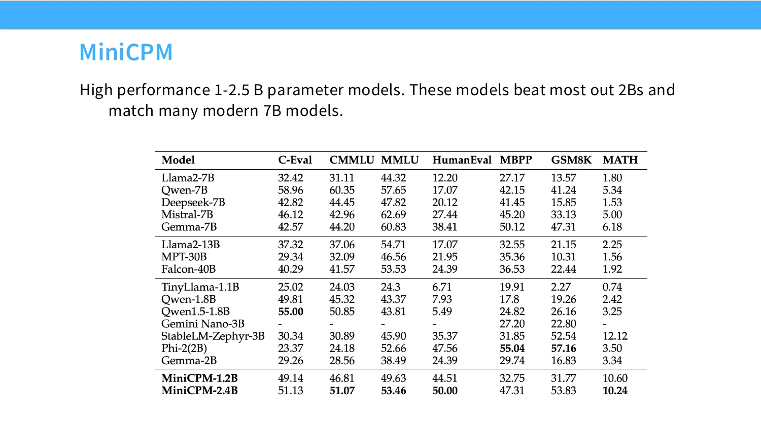
4:28 So mini CPM is an effort by, you know, a bunch of industry academic partnerships folks over in the Chinese open source community to come up with a high performance Smallish language model. And at the time when this came out, it was basically stated the art for like the one to two billion parameter bracket. Nowadays, you know GEMMA and other models, GEMMA, and other models at two B or three B are gonna be higher performance, but these are, you know, competitive, well trained models. At least those at 2024 standards. So, how do you train these models? OK, as I said before, you know, we have to get some of these like scaling parameters right, and one of the things that I'll talk about today, that I'll emphasize quite a bit. Is initializations are very important. Initial initializations are important because they allow you to make certain hyperparameters less scale dependent. So, the first technique that I want to talk about from this mini CPN paper, is a special class of initializations called mu p. #

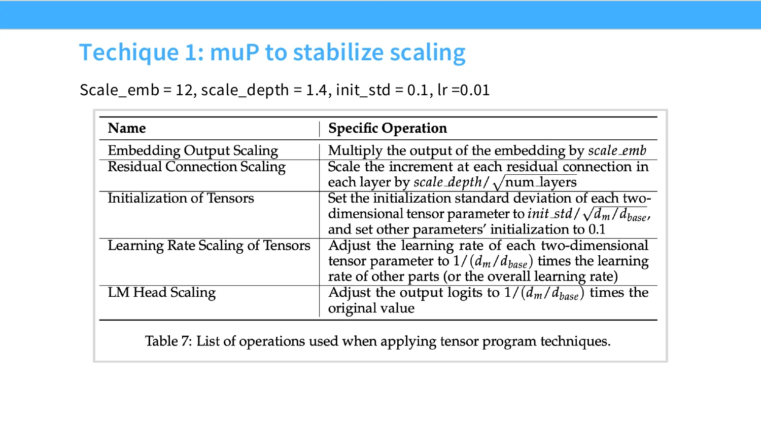
5:29 So mu p, the whole point of this approach Is to say, I want to make sure that my optimal learning rate is the same as I scale up and down, right? I talked about this very briefly, in in the two lectures ago, so you should hopefully remember that a little bit, but this is kind of the the first real instantiation that we're gonna talk about. What does that look like specifically? The mini CPM paper has a nice list of things you know to do. So they scale the embedding output, they scale the residual connections by the square root of number of layers. They scale the initialization of all their matrix shape tensors by the fan in fan out ratio. They scale the learning rates of tensors, and and you know you should pay attention to this one, cause this is exotic. If you aren't used to like per parameter learning rates, and then they also scale the LM heads. We'll talk about why you do these things or like how you derive this particular set of scalings. #

6:20 suffice to say that, you know, you're just going to change up how you're gonna do the initializations and your learning rates a little bit in the hopes of stabilizing your learning rates a little bit. #

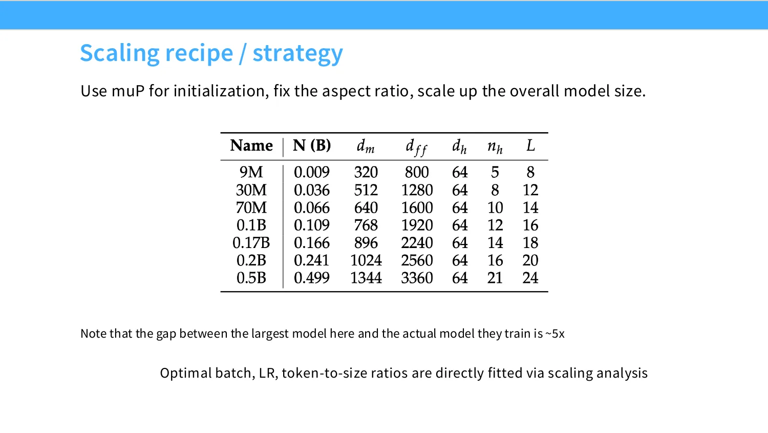
6:31 And of course we're training a small model here, but we're still wanting to do a nice scaling strategy, right? Like part of the point of the study is not that you want to brute force, you know, 1.5B model like training hundreds of them. You want to get the hyperparameters exactly right the first time, so you're going to train a bunch of much smaller models, and then get a scaling ladder up all the way to your target size. of 5 x or so, right? And so there's about a 5X gap between the biggest model they train on their ladder and the actual model that they're gonna finally release, right? And their goal is gonna be to nail down, I think what most people consider to be the sensitive parameters, like optimal batch size. Learning rate, and then the token to size ratio that we talked about a chinchilla, they sort of also wanna replicate a chinchilla analysis. Much less important to us, now and and probably to you, even if you're training. #

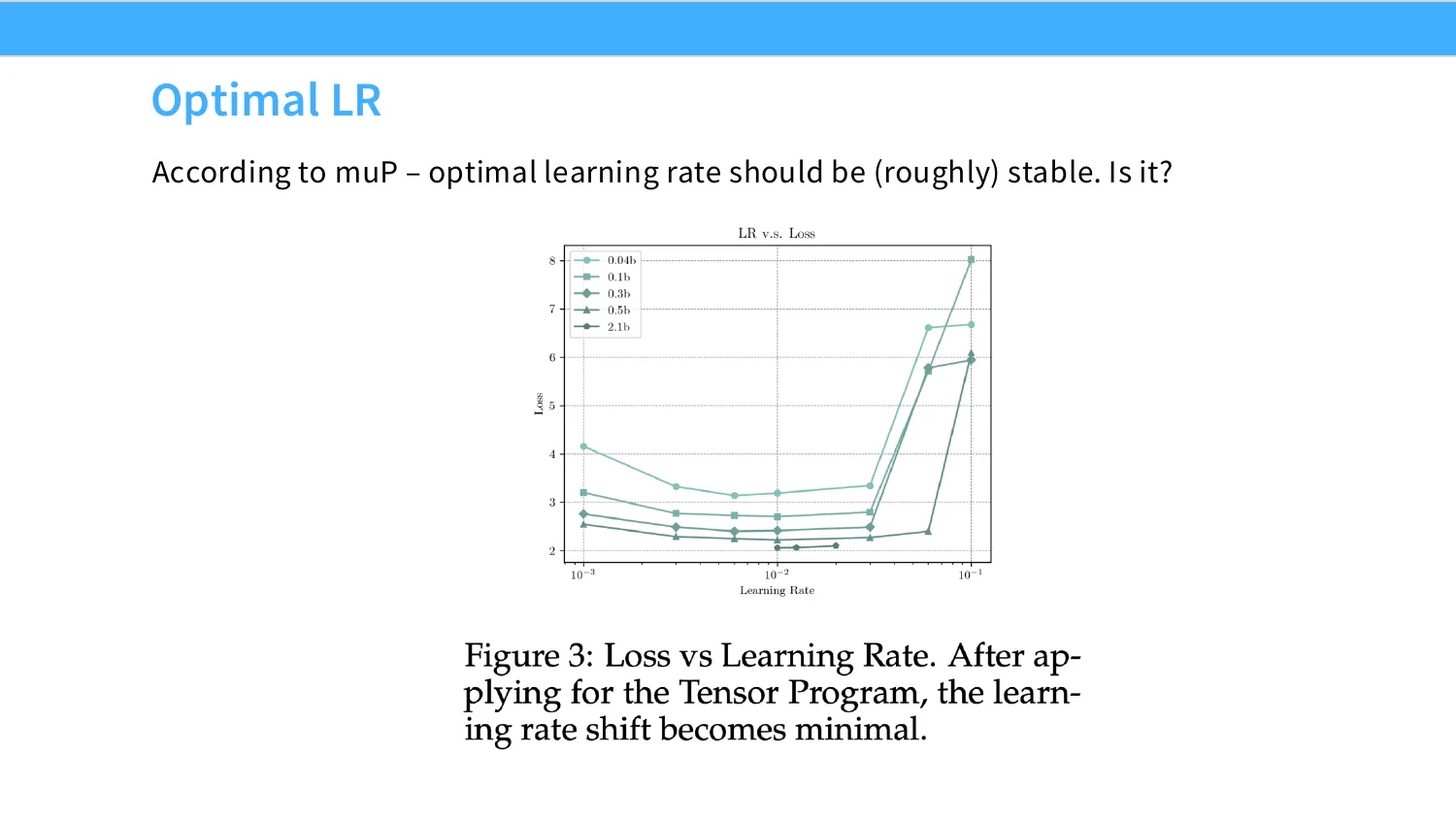
7:20 But I'm gonna talk about it regardless, cause there's one important thing in in the way they do that, and that I think is very informative and useful. OK, so as I said earlier, right, the whole point of going through this weird initialization or non standard initialization called new p. Is to try to make the optimal learning rate stable. Is it? At least in sort of the mini CPM case, the answer is yes. In fact, it's very very clean in their experiments. They sweep learning rate across a variety of models, so each line is a model size. The minimal losses basically right on 10^-2. I guess the minimum is slightly shifted for the smallest model. #

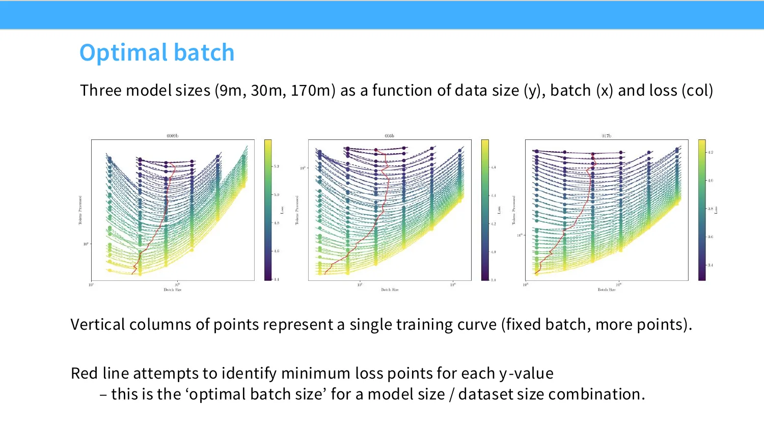
7:57 But I mean even then it's quite close to the minimum. So, this is you know a nice success case of the mu p approach. We will talk about several other models and other papers that use mu p. This is not the only way to do it, but this is one effective way to do it. And if you can get something like this, now you've kind of removed the need to tune the learning rate. But of course, even if you have a nice primalization that fixes your learning rate to a single sort of optimum, your optimal batch size is still not gonna be kind of the same. So the mo-, the batch size actually varies as a function of both data set size and model size. so in their case, you know, they run these sort of model training run. So each column of points that you see on these plots is a is a is a training run. #

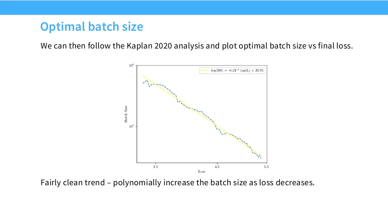
8:42 So they're, they have a fixed batch size. And they increase the number of tokens processed, I guess from bottom to top. And then they ask okay, we've done many of these training runs. What is the optimal batch size fitting sort of these quadratic sort of curves onto each of these sort of uhuh, lines over here, this sort of equal loss contour. what they find is sort of this kind of optimal batch size scaling as a function of the number of tokens processed, and they do this across different model sizes. You know, maybe you you would not be surprised by this, given you know the nice scalings that we saw in the Caplan paper for critical batch sizes. But the optimal batch size does have a sort of power law structure with respect to the target loss. And so we kind of see exactly the Kaplan style analysis of, you know, if your loss is lower on the left, your backside should be bigger, right? Critical batch size scaling. #

9:31 And so now given a particular loss target, which you can, you know, back out from the scaling loss. You can basically set what the optimal or you know critical batch size is that would give you the best tradeoffs, right? So, there's a nice clean trend here. This will let you set batch size very easily and precisely. OK, so those two, the batch size and the learning rate scaling, they're gonna come back over and over again. Those are arguably the most important and sensitive parameters to do scaling laws on.But. #

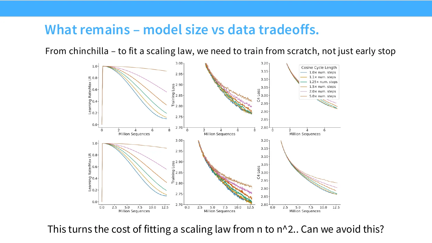
10:04 So, you know, remember like to do chinchilla, right? We need to train a lot of different models, so we're gonna let's say do isoflops, that means I'm gonna fix a flops budget, and I'm gonna vary you know my trade offs between number of tokens and model size. And to do that, I'm gonna let's say increase the amount of data I train on, right? So increase the number of sequences. But as I increase the number of sequences, remember that each one of these gets a different learning rate schedule, right? You know you all training on cosine learning rates. Cosine learning rates look different, you need to know the terminal sort of total budget before you train in order to have a cosine schedule, right? And so this leads the kind of a a annoying fact, which is that you just need to keep retraining your models. If you wanna train a you know 8 million sequence model, right? #

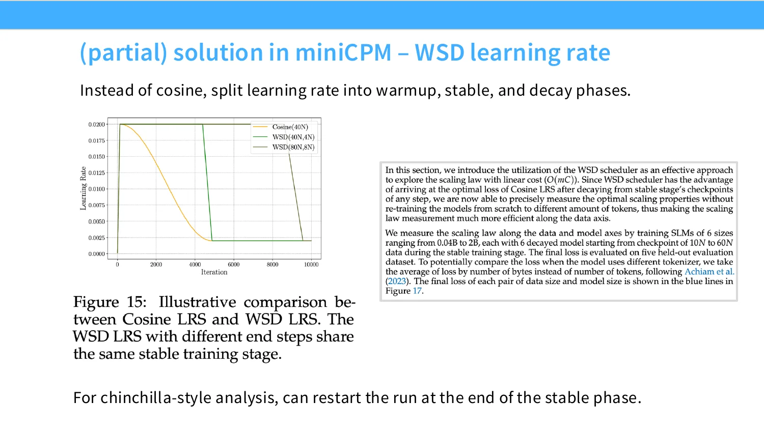
10:47 You can't start, like restart from the end of a 4 million sequence model, right? You have to just restart from scratch, because your learning rate schedule is just fundamentally different. And this is just very annoying. It's like a quadratic cost in some sense of doing this, because you have to keep restarting your runs just from the start. And this seems very wasteful. And I think lots of other people did too. And I think one of the nice solutions from the mini CPN paper is what's now called, I think the warmup stable decay learning rate, or this is you know the popular term for this. And it's basically a big trapezoid. So you've got a warm up phase. #

11:23 The warm up phase is usually defined as a constant number of steps, not as a fraction of your your training target, right? So this is independent. of your training horizon. you've got a fairly long run where you're holding the learning rates constant. that's the stable phase. and then at the end, you're gonna decay fairly rapidly down to zero, right? that's the decay phase. And generally, you know the decay phase is something like 10~20 percent of your total training run, right? So you're gonna be stable for the vast majority of training run, and then do a very rapid decay down to Usually about 10 percent of your maximum learning rate at the very end here. #

11:57 And that's like a a very typical warmups warm up stable decay learning rate. OK, and why do we do this? What's the point of doing this? Well, we do WSD because now we can restart a run at any point at the end of the stable phase, right? So if I want to reuse a run and like train it for longer, right, I'll just roll back my training to the vit lasts stable checkpoint, and then I'll just run the stable learning rates forward, and then red decay the model down to zero, right? So this provides a. very easy way for us to essentially run sort of scale in data experiments without constantly rerunning. your experiments, right? So you you do have to re-decay every time, but that's maybe 10 percent of the total cost. #

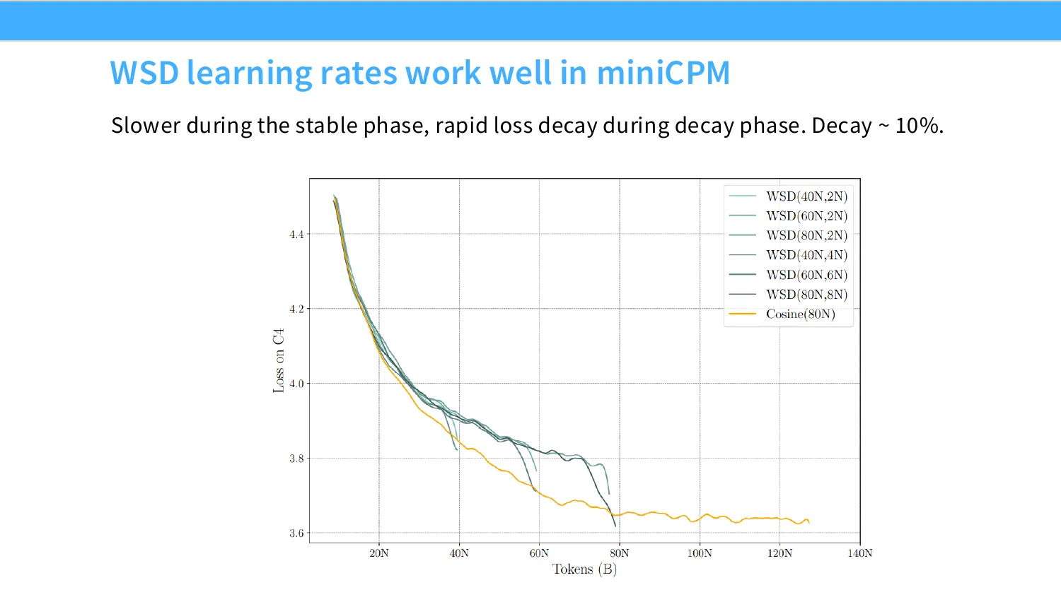
12:37 You know, it's a much better situation to be repeatedly decaying than to repeatedly rerun. Your pre training runs, and this is this is a very common trick that's used in many places. I'll I'll show, I guess a performance comparison. There have been many plots of this form. I think Who who was the most recent folks that were were maybe was Martin Jaggie and others. I think over at ETH had like an extensive study of like WSD sort of performance, but I think a lot of papers have shown similar things of, you know, you have a well tuned cosine learning curve. This is you know the orange line over here, and then you've got various WSD curves, and WSD curves always look a little bit funky. Because it looks like you're way underperforming until you hit the decay phase, where suddenly you kind of reclaim all of your gains, and then you sort of match or even sometimes exceed the cosine learning rate performance. Anecdotally, I think if you if you talk to a bunch of people training networks, I think a lot of people will say the cosine is slightly better in many cases. #

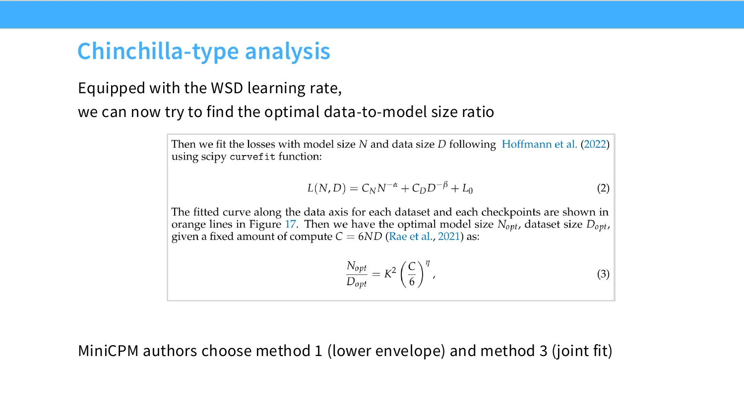
13:36 But WSD is basically as good in many other situations. Like it is a very versatile default learning rate. doesn't necessarily suffer from having to sort of rerun if you wanna just continue runs. It is very cool though to see, you know, just how much of an impact learning rate decay has if you haven't You know, played with that before, like it, this part of decaying the learning rate is just incredibly important to sort of getting the final sort. of unkneeling parts of your training. together. okay, so that's the comparison there. okay, so now that we're equipped with WSD style learning rates, you know, Chinchilla style analyses are actually very easy. What you're gonna do is you're gonna, you know, essentially run one long run, and then you'll just sort of rewind the checkpoints, and then repeatedly decay, and that will give you sort of sweeps along the data dimension. #

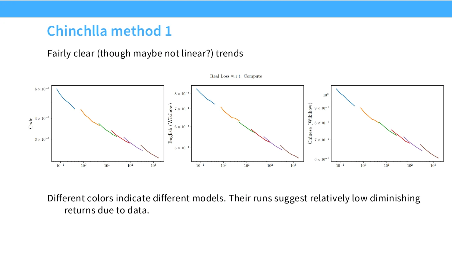
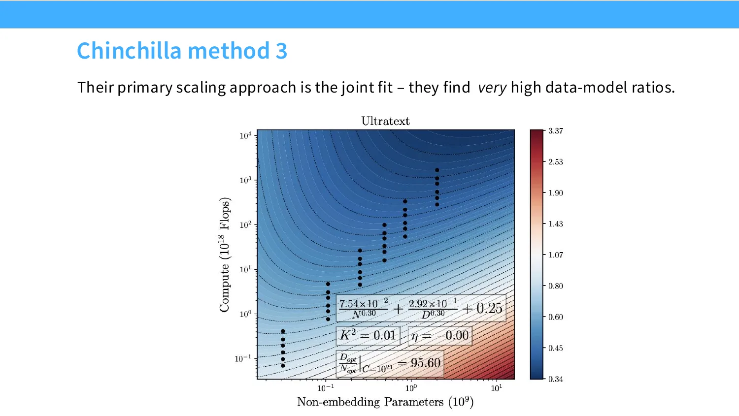
14:25 And then you'll also do sweeps along the model dimension. You can do iso flops or any other kind of analysis that you would like. The mini CPM authors for whatever reason choose to try to replicate methods one and three, which to me are the The least reliable of the ha Chinchilla methods, but you know they do get fairly nice looking scaling curves. If you look at the mini CPM sort of Chinchilla method one, they they see like nice Lower envelopes that look mostly linear across these, which is good. And then method three, they get nice smooth scaling for the most part in both sort of the the compute to non embedding parameter trade off. Soum, It seems like for the most part, they get reasonable tential looking fits. One thing I will point out, is that they get pretty different exponents for their overall joint fit. compared to Chinchilla, they claim in the paper that this means that they should be training with way more text pieces of text than Chinchilla. It is highly unclear to me whether this is a Really true or whether their chintz will fits are a little bit strange relative to the original chintz will paper. #

15:32 OK, I'll stop here for one moment in case someone has questions about mini CPM. Maybe the main couple things to take away is one is you know the use of mu p is a useful trick, I guess, to try to stabilize how your learning rate changes over scales. And the second thing maybe to remember is the WSD learning rate. That's just like a very common trick. You should all kind of know about this learning rate. #

03 DeepSeek：直接拟合 LR/batch 缩放律

15:52 That's a basic You know, thing to know. OK. #

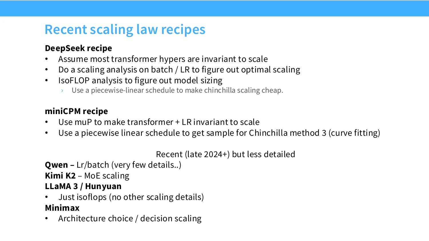
15:58 So then I'll move on to deepseek. This is the kind of you know original deepseek paper. Before you know they started talking about MoEs and all these other sort of very cool things. And I think even at the very first deepseek paper, you could kind of tell that these were very serious people, because I think deepseek llm, you know, even now, is I think one of the more nicely executed scaling analyses in the open world, right? And I feel like they have Lots of. great taste in the experiments that they run. So even before, you know, R one and so on came out, it was like kind of clear that these people were were going places. All right. So, Deepseek takes a very different scaling strategy than MiniCPM and and several others in trying to optimize their hyperparameters. #

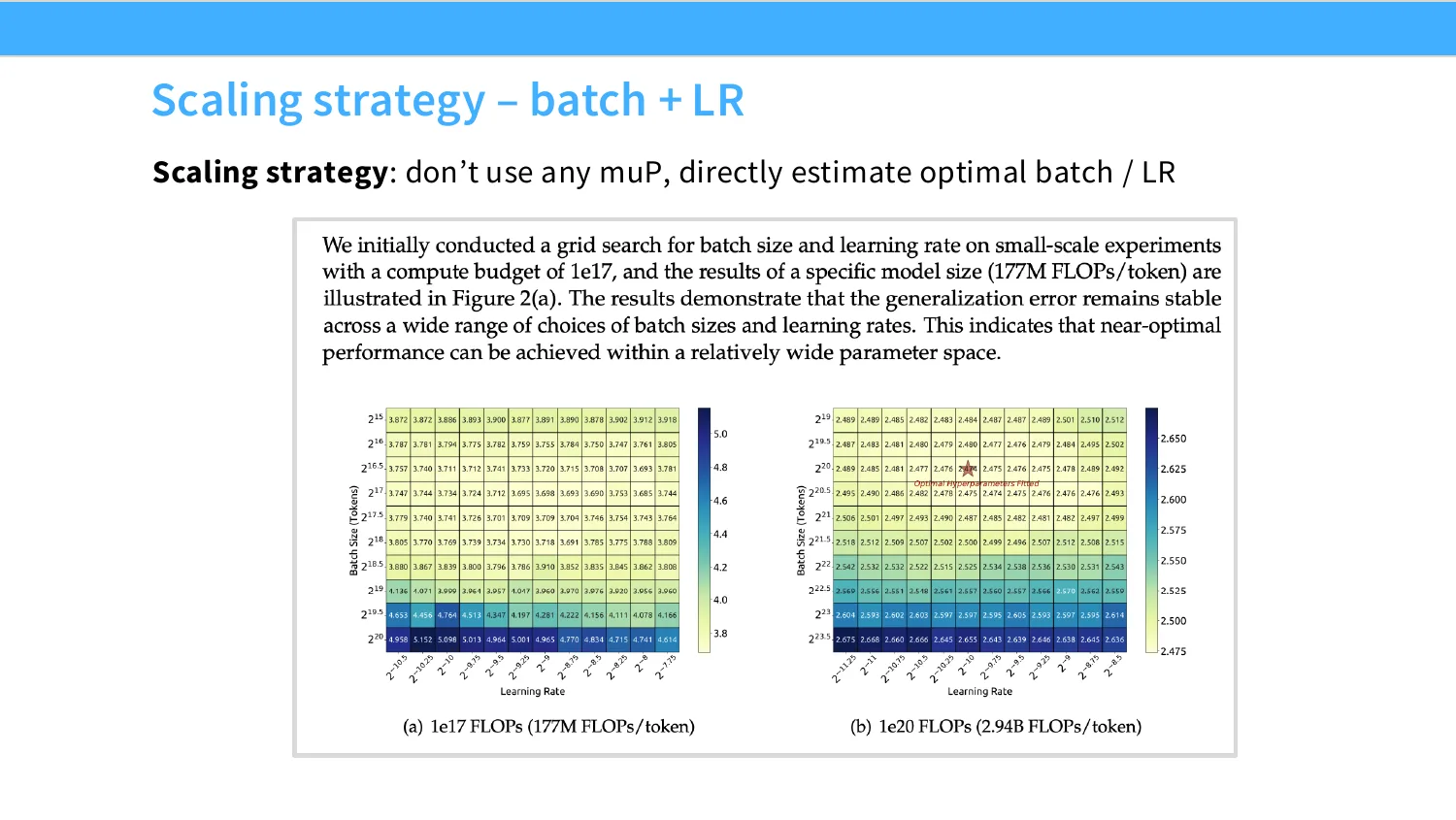
16:43 Like, they're not gonna really do mu p, right? They're not gonna do this like interesting Scaling adjustments. Instead, they are going to directly try going to try to fit a scaling law to estimate both the optimal batch size and the optimal learning rate, right? So, we know that the learning rate and batch sizes should actually change with scale. But if the way in which they change are predictable, just like a scaling law, then we're good to go, right? Like we don't really need to to worry about very much. So what they do is they basically run extensive grid searches at very at various different scales, and they try to find the optimum, right? So this is an example of the kind of thing they're doing. You know, they're sweeping learning rates, they're sweeping batch sizes, and they're looking at sort of the terminal loss. #

17:24 If they're processing a a particular number of tokens, right? So they fix the compute, and then they vary these two. They'll do this across several different scales, and then they'll basically try to identify what the lowest losses, in this case the lightest color, right? So they they'll put a little star there. And then they'll do this across scales. So if you do, you know, this across sufficiently many scales, you will get a plot that looks look like this, right? And this plot is saying okay. I'm going to vary my non embedding trading flops across some range, and you can kind of see these gray dots over here, right? And I'm gonna vary, as I vary this, my optimal back size will change. #

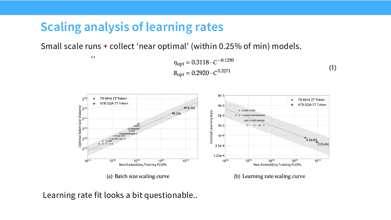
18:03 Re- remember the optimal back size is derived by looking at these big grids, and and kind of finding the minimizer, right? and I will get something that kind of looks like a line, right? The optimal backside should scale with my non embedding flops. I'm in similarly for my optimal learning rate, right? I'll get a bunch of gray dots in my sort of non embedding flops range. And then I can fit a line to that to try to estimate what my optimal learning rate should look like. So, this is fairly nice. And I guess one thing I'll point out is, you know, their their full runs are on the star, right? These are the runs that they chose, at higher flops, they they have much higher batch sizes, and much lower learning rates, right? #

18:47 The stars are the things they actually ran for their their big runs. These fits look reasonable for the batches, right? This kind of does look like a line. The one on the learning rate, I I'm not quite sure. That constitutes you know the best linear fits that I've seen in my life. But I guess it works, so it's probably fine, right? Like the models do train, the models do get reasonable things. I think this is the one I would say like drawback of the learning rates approach, it's not really clear That if you try to do this grid search kind of thing, unless your grid is in the right place. you've got a lot of quantization error, and then you're not getting very good scaling law fits, and you end up with kind of something that looks like an arbitrary linear thing going on. #

19:30 OK, oh, yes, sorry. #

19:33 Welcome for the same number of training flops, there you get multiple data points with a large range of optimal version. Why is it that you get a large range of optimal learning rates for different train flops? Is that is that the question on the y axis over here? Yeah, so the the reason I think there is because of the the changes to the model sizes and things like. #

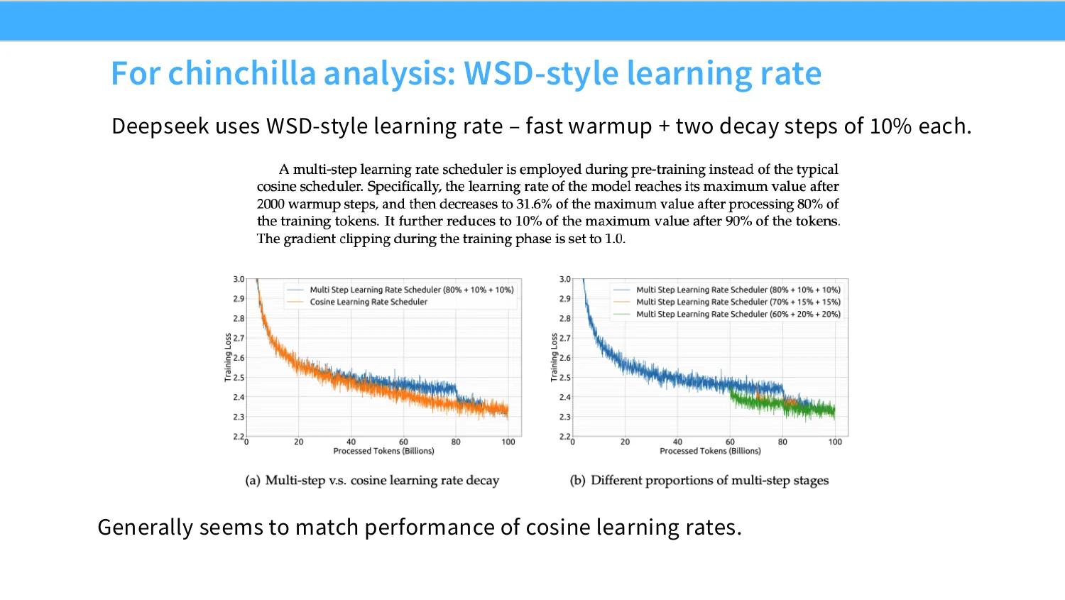
20:01 And so, you know, the 2024 was back in the era where I think every open model builder was replicating the entire scaling loss stack. And so, you know, deepseek also complements the, you know, like like learning rate analysis with basically a channel replication. And to do that, they're also gonna do the same thing as mini cpm. They're gonna follow the wsd style learning rate. They have a weird little variation where they do two decay phases instead of one. I am not really sure why this is. It hasn't really been a thing that has taken off afterwards, but it is a thing that they do. Regardless, the whole point here is to say WSD is an effective approach, and you can use that to replicate Chintala. In deepseek, you know, has much nicer scaling curves. #

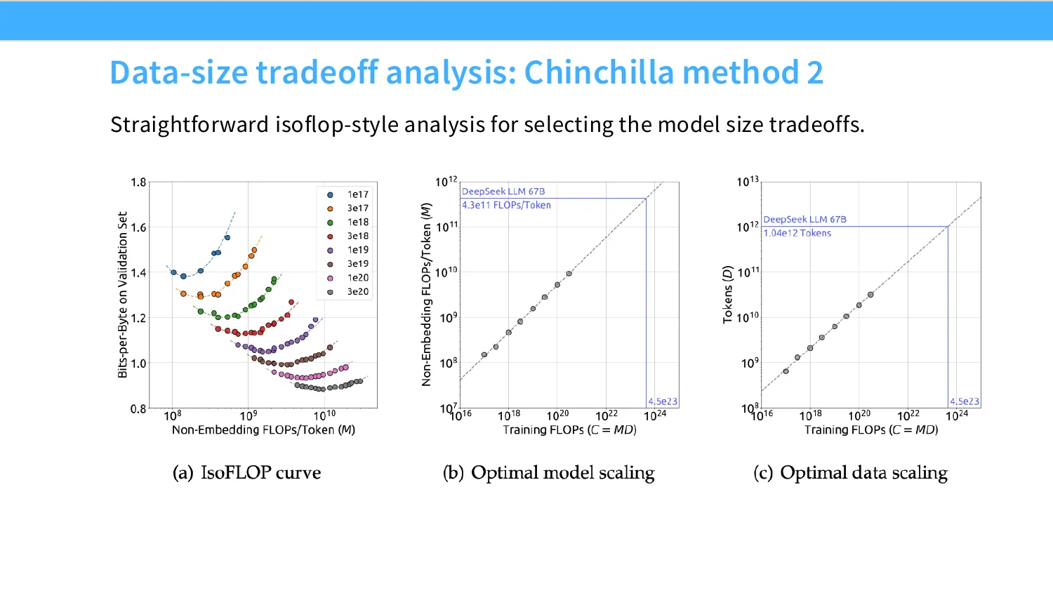
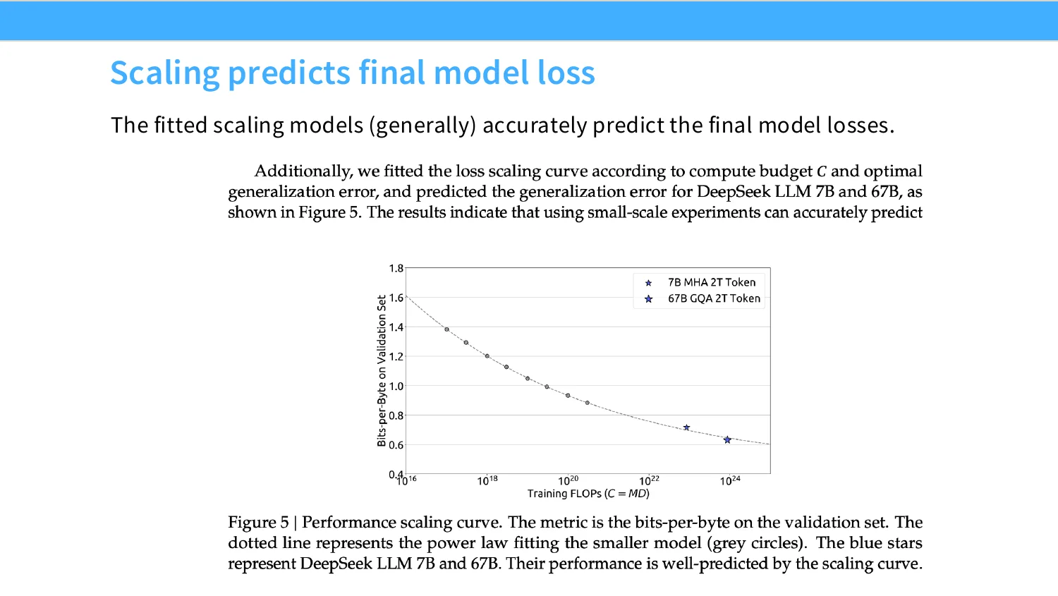
20:50 the mini cpm, because of their choice to go with isoflops, so they get these very nice, you know, clean sweeps on across the the fixed flops ranges, and then they also get fairly nice and clean chinchilla style trade offs. as before. so this allows them to essentially replicate the chinchilla results, and get you know a similar kind of of a data model scaling law. really the point that i'm showing with this is just to say look. But in Chile, laws have been replicated by other people at lar- large-ish compute ranges. So that analysis is generally sound. Finally, I think you know this is kind of the I I'm a little bit sad that these kinds of pots are now somewhat rare in open source release papers. But you know this is really the the final punchline of a lot of scaling law work, right? You train a bunch of small curated models, you know, at smaller computer ranges. #

21:42 And then you kind of like draw out the power law, and then in the end, you get something pretty close to reality if you scale out enough, right? So the two stars are the models that they actually trained. The great odds are their scaling law fits, and they're getting like pretty good predictions on their star. I mean it could be better, but it's not that at all. And so, they're able to get some pretty accurate scaling law predictions. on real, you know, open source models that face. OK, I'm actually I'll stop here. If people have questions about the deepseek stuff, feel free to ask them. I think my one line summary here is to say, you know, this is the other approach. #

22:18 To dealing with the sensitive hyperparameters, you can either attempt to stabilize them, or you can attempt to just scaling law fit them, right? And then just go with the scaling law. #

04 其他模型的经验：Qwen 2.5/3、Kimi K2、Hunyuan、LLaMA 3、MiniMax-01

22:26 And deepseek it represents them more like fit the scaling law approach to this problem. #

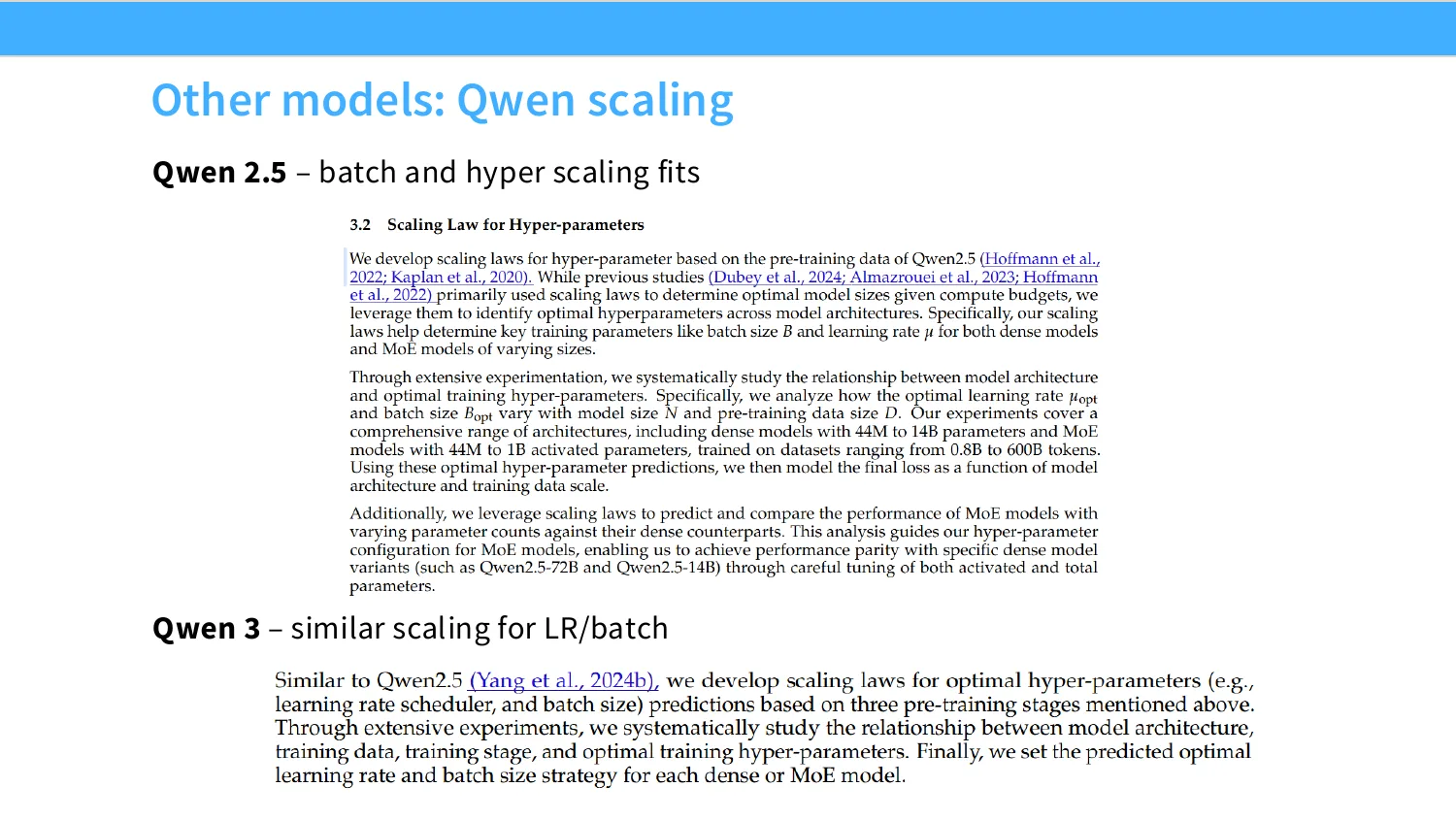
22:32 Good, OK. So, there are other models, more recent ones that have, you know, nice scaling laws that they talk about. As I said before though, I think a lot of this work is now, you know, kind of, wha- what's the, it's kind of like all known to everybody, and so no one is really putting a lot of this stuff into like big sections into the paper. So if you look at Gwen 2.5 They say something like, OK, well, we need to tune some optimal hyperparameters like batch sizes and learning rates. So we do a bunch of scaling experiments to figure out what the optimum are, and then we have a scaling law, and we predict the optimum, and then we're able to do that even for MoE. Right, so this is basically the same thing as the deep sea analysis, right that they're talking about in Quant 2.5. Same thing with Quant 3, right? #

23:18 At by the time it's Quant 3, you know they say, alright, we've already figured out what to do in Quant 2.5, we're just doing exactly the same thing, right? So this has become part of a very standard recipe. that you use in order to nail down the optimum optimal learning rates and batches. #

23:34 Kimi K two is probably the newest paper that I'll talk about of the series. At this point, I'm just gonna quickly go through several papers, maybe need to give you sort of a overview of what people are doing. In terms of scaling work in the in the open source model releases. So, Kenny K two and a few others have focused on essentially M O E scaling laws. So, you know, it's 2026. Most people know you know how to do a tencent scaling law, or even a learning rate scaling law. What things are new? Well, a lot of these companies are now switching to M O E s, fully switching to M O E s, right? And if you're doing that, you really want to know, you know, am I training the right amount of active parameters? #

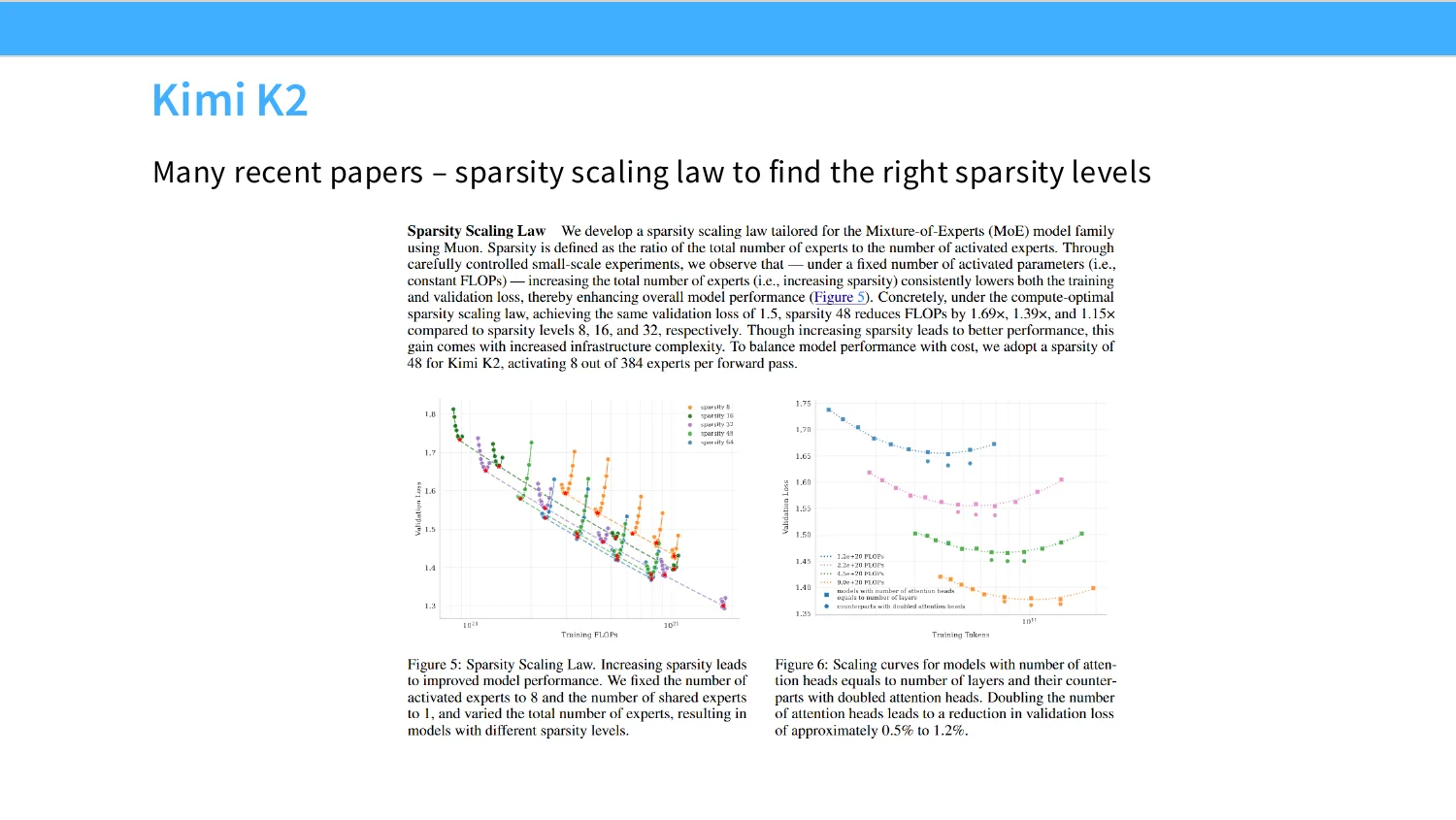
24:14 And so, they're doing things like, okay, we're gonna vary the flops, and look at my losses, and I'm gonna do so for different levels of sparsity. so that i can figure out how much sparsity helps or hurts my losses. and their conclusion of courses as if you look at the different sparsity levels, the more sparse your network right, the better your validation loss. Given a flop, unsuprising, but now the fact that they can quantitatively know what the relationship is between sparsity and loss means that they can make sort of more rational decisions about you know how much sparsity to put into their model, and they they look at this and they say okay. What we're. gonna do is we're gonna use a sparsity of 48 because at that point we're hitting diminishing returns on our scaling loss. So, you can kind of see how this kind of analysis is used to justify different architectural decisions across different open source releases. Honyun, which is another open source M O Euh, From few years ago now, they do a very similar thing, right? Like, I think every company once they switch to the M O E has to do this kind of like a M O E scaling law to figure out how the number of activated parameters or the amount of sparsity Changes training loss, and then they kind of redo a lot of these analysis. So, for. #

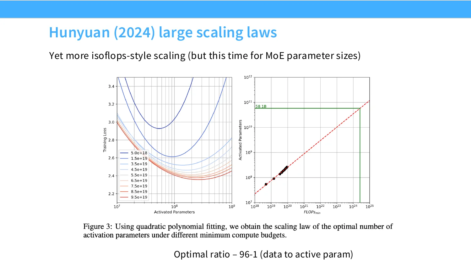
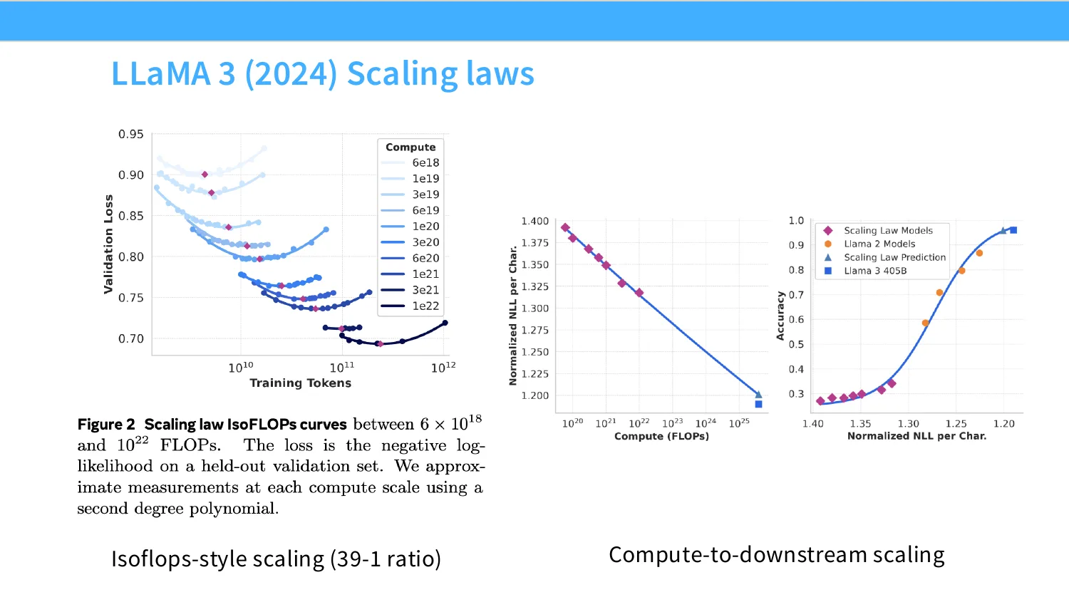
25:26 example, in in Honeynet's case, they end up with like a 96 data point per active parameter ratio. In their case, they're fixing the sparsity level, and so that that's not a thing that they're searching over. Lamba three also has some nice scaling laws. Unfortunately, they're not particularly useful ones. They do isoflopped style scaling and and get slightly different but similar ratios. For token to model, the most interesting thing that they do in terms of scaling in llama 3 is the the plot on the right here, which is you know they have the usual scaling law. which is the left panel, that's saying i if I have more compute Then the log prob on the the sort of answer for a benchmark sort of decays consistently. And on the right side they show, OK, well, you know, if you have better sort of log loss. Then the downstream accuracy also goes up, right? #

26:18 So they're basically saying well, we can just fit a sigmoid on these purple points, and that might give us a sense of like how good these different models are. You can kind of see their systematic deviations from the curve, so I don't really know If I would really buy that this curve is like the one truth that's going on, but you can certainly see that it is consistent with a sigmoidal scaling. mapping from the loss to the accuracy, which I think is very useful, right? Because we've been talking only about Kind of log losses, but there is a tight coupling in some cases or many cases between log losses and downstream accuracy. #

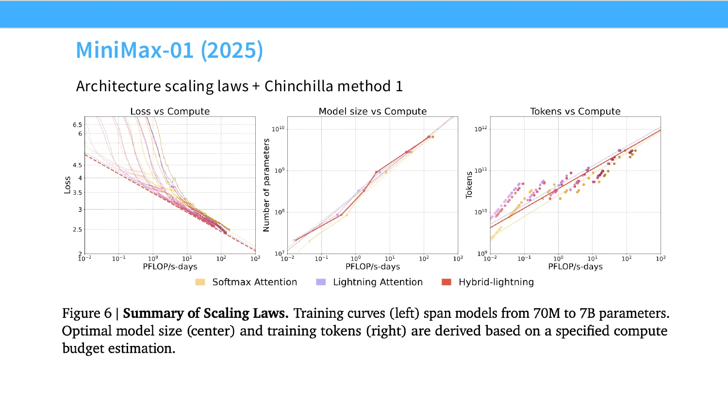
26:53 OK, and then sort of for one last paper that I want to talk about for scaling, Minimax 01 from last year had this nice set of scaling experiments where they were doing the exact kind of thing I was saying.is a useful affordance of scaling from two. lectures ago, and that is architecture variations. And so, they wanted to understand, okay, I have lightning attention, which is like some kind of li- a linear attention architecture. I have a softmax version like full attention, and I have a hybrid version that mixes the two. How do these things scale? You know, is it the case that if I scale up, one of them will get much worse than the other? And so, you know, you can kind of see this, they're replicating essentially the Kaplan plots of like, as I increaseuh, flops, you know how do the learning curves change, and you know is the number parameters that I need different for different levels of compute for these different architectures. And. #

27:47 the answer is for the most part kind of no. That you know, hybrid and lightning and softmax are all comparable for the most part, and they require similar model sizes. And this set of plots is used to justify their use of the hybrid architecture. In the actual deploy system, right? So this is exactly the kind of decision making that you would do based upon a scaling law. #

28:09 So, that's basically what I wanted to cover for the the recent scaling law recipes from the various companies. So, the two things as I said before, for the deepseek recipe right, really the key thing is the scaling analysis on the batch and learning rate. This is the scaling based approach. And many CPM follows a more of a mu p style approach to to try to get in variances. And then, you know, we see some trends. We see that like Kimmy and Quinn and others are do or in Huyuan are doing these like MoE scaling experiments as they switch to MoEs. We see some architecture work by a Minimax, And we also see you know some isoflops analysis being replicated by several others. And the to return to a previous point right, the point here is, I think a lot of companies are now less detailed, because the core scaling machinery like you know doing cichilla or doing learning rate scaling is now fairly well understood by everybody. so there's no Necessarily va-, ex-, extra value in you know showing those experiments for some of these releases. #

29:07 The or at least that's my guess for why we have much fewer of these kinds of experiments in the release. OK, I'll take one minute, and then sort of pause and let you digest and ask a question or two, in case you have questions for this part. #

29:27 Oh yeah. So all these cover the the pre training stage. So my question is what changes and what do not change when now pre training is kind of standardized process for all the Yes, the question was about what have, what changes about this when you do, or when you think about post rating, I guess, broadly. I think that's. still a big open question. There's no great way to do like fully integrated scaling with like post training accounted for. Because post training like can sometimes really change the nature of like. #

30:02 The closest things that I can think of to thinking about post training. is, there's been some work on like understanding like coverage or like you know diversity notions in pre training that would help predict what happens in post training, but it's still pretty nascent work. #

05 StepFun：LR 与 batch 的实证缩放研究

30:17 I don't think there's any good Answer to the question of like what do we do about, you know, synergy with post training. #

30:26 OK. #

30:29 So now we're gonna talk about the other piece. So, I think the two remaining parts of this lecture, kind of map on cleanly to the two examples. So, I'm gonna talk about one approach, one set of approaches, which is about scaling laws for learning rates, batch sizes, and optimizers, right? That kind of corresponds to the to the deepseek approach to the world. And then I'm gonna talk about kind of the mupe stuff, right? Like the, that's kind of the mini CPM approach to the world. Can we just reprogram tries everything to make it so that we don't have to worry about scale? So We're gonna now talk about kind of the deepseek approach. How do we scale learning rate properly? #

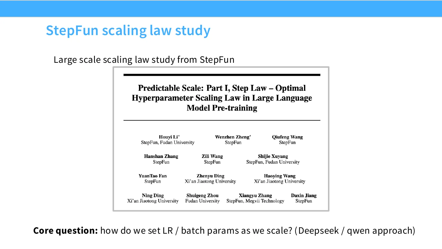
31:07 And so, there's gonna be a hyper parameter part and an optimizer choice part. And I'm gonna draw quite a bit from this pretty recent preprint, from the STEP fun folks folks. I don't think there's like a great, you know, really truly like reliable, robustuh, Study on hyperparameters, especially learning rates. But this is probably getting somewhat close. The steps on folks train, you know, credible large models and release them, and they burned a ton of compute in grid searching the space of hyperparameters in the scaling law studies. So I'll go through this and like, you know, show you some in- intriguing empirical phenomena. About how learning rates, batch size, and all those affect downstream losses. #

31:51 OK, so lots of people have talked about lots of different ways of scaling learning rate and batch sizes as roughly as a function of compute. And you know the stepfun survey, not survey paper, the hyper primate tuning paper has this very nice table that like captures a lot of this. And I'll point out a couple of different things. Some of this we already know. So, the very top row, this OpenAI scaling law, this is from Kaplan. If you look at the batch size over there, notice how it says like two e eighteen. You know, capital L to the exponent, that's critical batch sizes, right? It's basically saying, you know, you should scale your batch sizes as a function of your terminal loss. Great, right? #

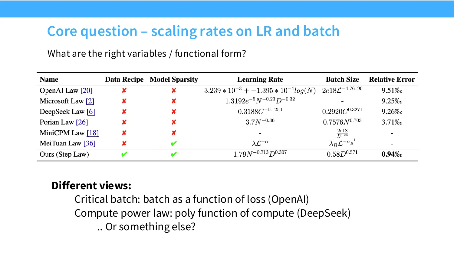
32:32 Deepseek we just saw, right? This is kind of the the compute based scaling loss for both learning rate and batch size. I mean there's been a couple of other folks that have proposed various kinds of scaling, including mini CPM which we talked about as well. You know, another important thing that I want to point out is that these, you know, formulas for learning rate and batch sizes, they don't even have the same inputs, right? Like people don't even seem to agree, what are the variables that should affect these learning rates? Like, you know, the OpenAI one is terminal loss. Whereas the the step fun folks, they claim that the right batch size scaling is a function of the data. Right? So there's a lot of different sort of disagreements about the nature of scaling for hyper parameters. #

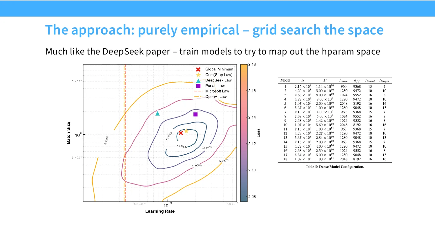
33:14 And I think one thing I'll say as I go through this is not to take even this last row as kind of gospel, right? A lot of these things are are pretty brittle in many ways, but the experiments and the phenomena are things that you can learn well from. So I'll do that. So the design of this paper is very similar to the deepseek one, like they're just gonna train a ton of models to you know grid out both the learning rate space and the back size space. and do them across a range of models and range of data set sizes. And by doing so, they they hope to essentially saturate the hyper parameter space for a set of small models, and then nail down what the optimum is. And much like in the deep sea design, they're going to be, you know, after they grid up the space, you know, in this case they have a contour plot, but the underlying objects are just they run a bunch of models. They aim to try to minimize sort of the losses, right? And the control plots are quite nice, I feel like they give a good visualization. #

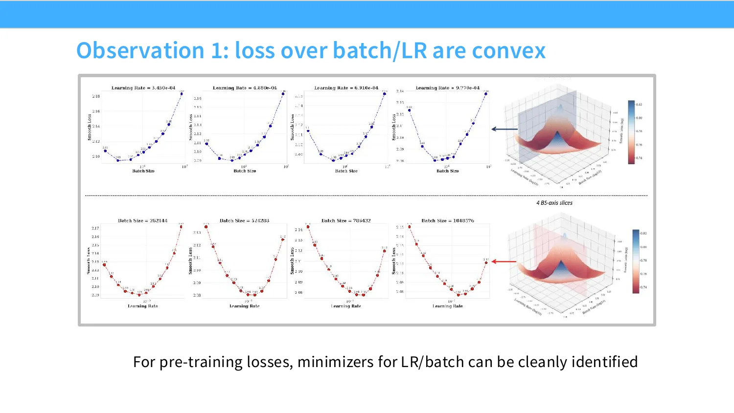
34:12 They ran a pretty high resolution grid, and thanks to that, one of the things that we can see is that they can actually plot out a fairly high resolution contour of what the hyper parameter space looks like. In this case, this is a slice At one B parameters and a hundred B tokens, I believe. And you can sort of se- see on the right side that surface is the hyperparameter sort of landscape, you know, as a function of the batch size, which is kind of your one axis. and learning rate, which is the other axis. How does the loss change if you fixum, The total amount of data in the model. Now, you know we see that each slice, like if you fix a batch size or you fix a learning rate, right, each slice is kind of nice and convex, and it's almost even smooth. And this is quite nice, because it means that you can, you know, kind of search for the optimal hyperparameter, you know, fairly nicely, and you can be confident that the minimum is not too far off. This was very jaggedy. You might have some you know very serious doubts about whether this kind of program of gridding the space is even viable. #

35:13 Also, this should maybe give you some nice intuition about the smoothness of the hyperparameter space in general. And I think there's actually one really interesting general scaling trend. And looking at other related papers to this topic, I think, I don't know if I've seen any contradicting evidence to this. observation. So, I think the one thing that seems very interesting, and one of the key takeaways of this work, is essentially if you're looking at the optimal batch size. Right, the only thing that seems to depend on is the total amount of data that you're training on. So this right hand plot is the is the one to look at, right? So x axis here is the amount of data that you're training on, the different color dots, those are different models. Notice how you know the different color dots seem to follow roughly the same trend line here, fairly predictable one. #

36:01 And this is in log log scale, so you you should expect some sort of a power law as a function of d. On the left panel, we have the dependence of learning rate, and we see that this is a very different behavior, right? Bigger models, so if you go from blue all the way to this pink color, right? Bigger models have smaller optimal learning rate, and larger amounts of data have higher optimal learning rate, which is kind of counterintuitive actually. And so this might be a little fragile. There are other kinds of papers that argue that the dependence on D should be kind of reversed. But the trends here at least on this experiment are quite clear. #

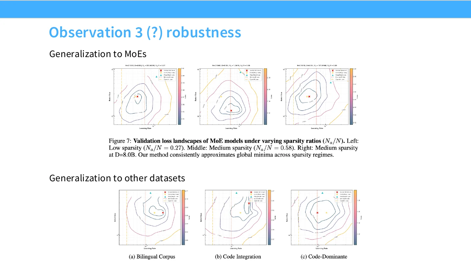
36:44 And you know, one final thing that I kind of want to point out is the learning rates are actually pretty robust, and I think this is backed up by a lot of experiences and experiments that people have. You know, I think people have a sense of like, you know, actually, as a poll, like, do people know what a good like hyperparameter is? Like, if you were told to train a language model tomorrow, like, would it be one e negative three, one e negative four? Right, I feel like we roughly have a sense of like, actually, this range of hyperparameters for learning rates. Is generally a good starting point. And that is generally true. So so the scaling laws that they got, you know, actually transfer over to, for example, M O E's, to a to a certain extent. The yellow stars, which might be a little harder to see, are the predictions from their scaling laws. The red Xs are sort of the optima that are derived sort of directly on the MOEs. #

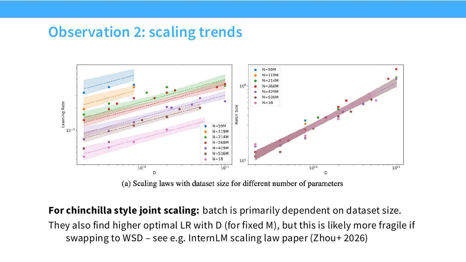
37:34 And so, you know, you switch to an MOE, you don't end up with a very different scaling law, as long as you're roughly controlling for active parameters. The one thing that does seem a little bit more, you know, potentially dicey is, you know, as you shift the training data, the optimal learning rates and the optimal batch sizes do shift a little bit, right? Which means that all of these phenomena are likely contingent, like the specific numbers that are are in the scaling laws and so on. Are potentially contingent to the data that you train on, more so than others. And so, I wanna flash this backup, you know, before I sort of move on. Right? So, you end up with some sort of simple scaling law at the end, which says, okay, batch size You know, maybe should be roughly square root of the number of data, times some constant. Your learning rate should kind of scale, you know, upwards with that side or upwards with data, but downwards with the model size. And that's kind of a surprising effect. #

38:29 But you know, not maybe crazy, because these experiments often in many cases are assuming like chintel like scaling, in which case, you know, those two would kind of cancel, and as you increase compute, your learning rate should go down. I'm hopefully that Chinchilla comment was clear. What what I mean is when you're scaling by Chinchilla, N and D are sort of both driven by compute, and as compute goes up, you expect your learning rate to go down, right? And so you will end up with something like the DeepSeaClaw. Where the learning rate decreases with compute, and the batch size increases with compute. Or, I'll be it with different exponents, than the deep sequel. #

39:03 Cool. #

39:05 OK, so in some sense this is like the the newest and most large scale version of the deep sea analysis, and this is one way that you know if you were doing the scaling law style approach, you would approach this problem of fitting a learning rate. OK. #

06 优化器与尺度依赖

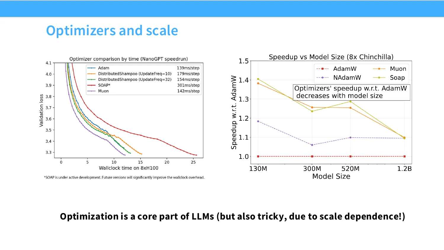
39:22 so, you know, that's the hyperparameter story. If someone has questions, feel free to stop me. And then next, right after, I'm gonna move on to Talking about optimizers, I think this is one thing that I, you know, didn't have time to talk about in the in the architectures lecture, that was already a pretty packed lecture. But I think it it would be sort of a disservice. to you, if I don't talk about optimizers. And optimizers are scale dependent, so this is a good place to put them and talk about some of the latest and greatest developments in optimizers, and their relationship with scale. #

39:55 Oh yeah. So, I guess like, the, trying to figure out. #

40:09 Yeah, I mean, I think it depends like what regime you're in. The question is like, oh, sorry, I have to repeat it for the online folks, right? Is you know, should we just take the scaling on and run them, or like, should we just do our own grid search? You know, it does kind of depend on the amount of compute budget that you have, and how much you need to nail it. I do think for example, you know, maybe the step fun law, if you're in the right compute regime, like close to where they were running the grid. These are probably really good defaults, right? Like, I would bet o- on these over like something I pi- pull out of my hat. That said, you know, if you were doing your own big pre-training run, you are probably gonna have minor differences, right? Like, you know, someone might say I really believe we should have a big weight decay. #

40:48 My architecture has a big weight decay. You know, we don't know necessarily that those things are gonna scale the same, right? And so you might want to actually redo a lot of this, and this is why I think a lot of the You know the the reports I showed you were redoing Chinchilla, redoing all these things. because there's enough minor differences that people want to check and make sure that they're like roughly first order correct. with these results. I think this will come up again in this next optimizer part, and I was talking about this with earlier, which is, you know, scaling laws kind of have this very scientific feel to them, it's like. oh, yes, stick these lines and extrapolate them, but ultimately a big part of scaling laws is still vibes. Right, it's like, do I really believe that the experiment setting of this step fun survey is similar enough to mine that they will transfer? We can't possibly know, right? #

41:34 There are always tiny differences. #

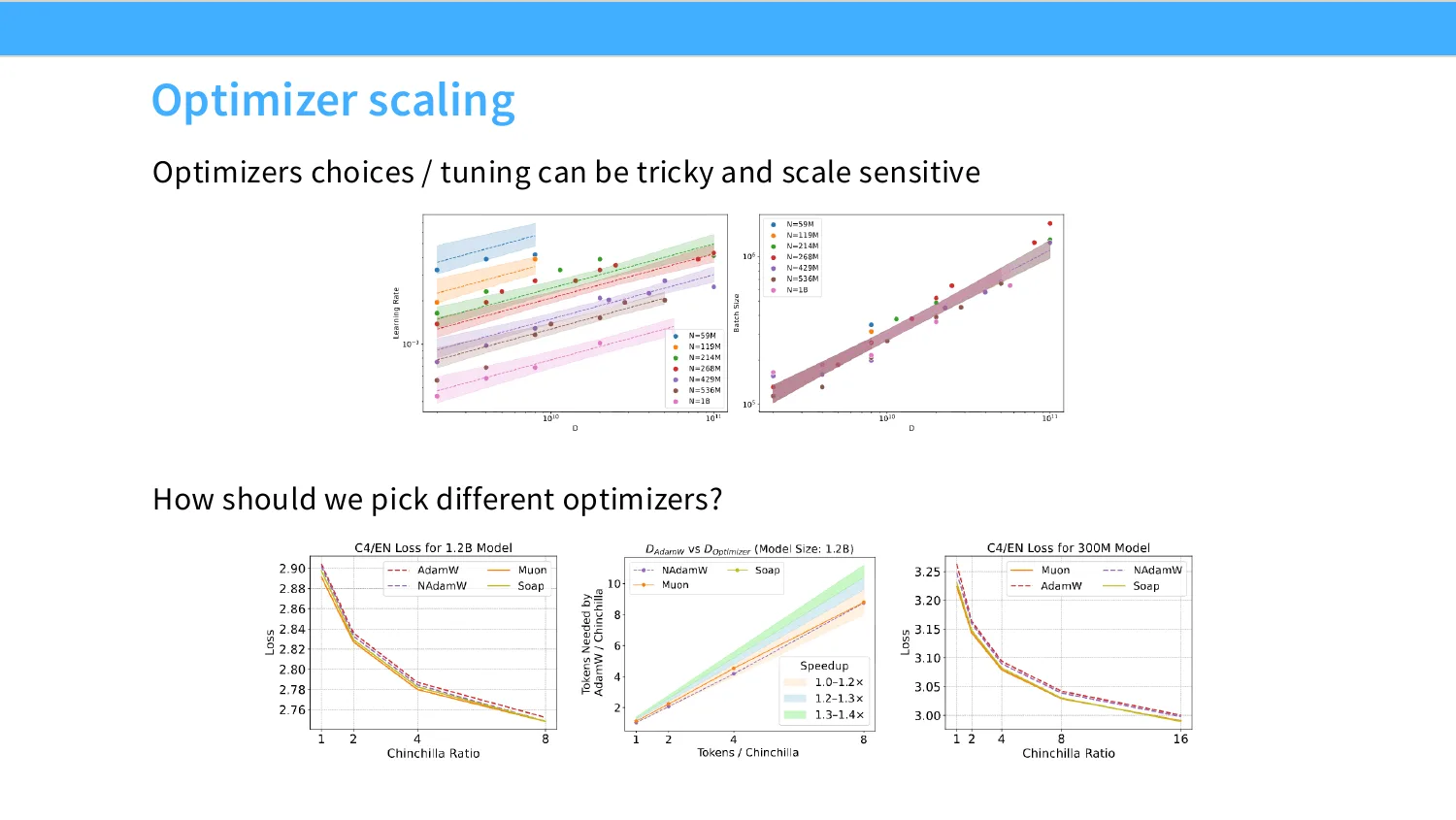
41:40 Good. OK, so now I get to talk about optimizers, and I think there's been some really exciting developments in LM optimizers, and maybe even deep learning optimizers in general over the past Year or two, and so this is a exciting time to talk about them. And so kind of the. story that I wanna start with, and and one that like should maybe motivate the subsection. Is this comparison over here, or maybe we'll start on this left panel, right? So, this is from nano GPT speed run, which you know inspired our assignment one. And there, you know, you have a really tiny tiny model that you're training on a fairly short amount of time. And you want to get to, I forget three point some loss as quickly as possible, right? And you know many people have been hill climbing on this benchmark, and I think one of the more, you know, remarkable things that have happened on the benchmark Is a as a benchmark called mu on. #

42:30 in in purple over here came, and you know got really significant gains over Adam, which is blue. It's right underneath the green line over there. So you know you you can just look at the green and the purple and that gap, and you say wow. You know, lots of big gains from just changing the optimizer to this mu on thing. And it's not even slower than Adam, much slower than Adam. That's great, right? But then, you know, there's a question of like, well, is this thing actually good at scale? And then you go and run some like scaling studies, and maybe they're not quite as good. You know, this is a really tricky and important part of how we do research, right? #

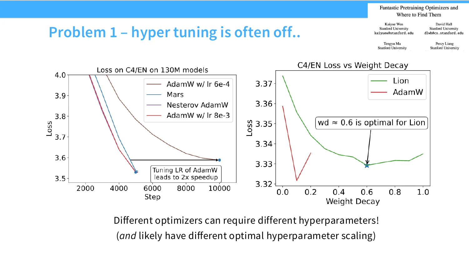
43:04 We have a small scale experiment, we have something that scale dependent for sure, like an optimizer. And then we see really big gains in the small scale, what do we do? About the large scale, and more than providing like a solid concrete prescription, I I want us to maybe almost even provide a story here, so that you can kind of get a sense of like what we can do, and what things we can't necessarily know. OK, so, actually, before I move out the next slide, you know, and and this kind of thing happens all the time, where you like come up with a great thing small scale, and it just doesn't maybe pan out large scale, so what's the difference? I'm gonna spend a few slides talking about Kayia and and sort of Tangu and Percy and David's paper, basically doing a large scale set of experiments on Comparing optimizers, and do, trying to do that comparison better. I mean there's a lot to learn about. scaling and other things from that, but also just standard deep learning stuff. You know, there's really basic things like You know the hyperparameters for different models are different, so if you're scaling things up, maybe they even have different scaling exponents. So you have to tune Adam really well. #

44:09 So if you tune it badly, you know you get this this darker brown line, and you're like, wow, this thing is much worse than all these other algorithms that I have over here on the left. But then you you change the learning rate a little bit, and you're like, wow, actually all my gains went away. Similarly on the right, you know you can have cases where maybe you've tuned your learning rate well, but now you've got other stuff like weight decay that is not optimally tuned. And so if you use the same weight decay, then you're certainly gonna get a much worse result for this green line, right? If you pick this, you know, small weight decay, you'll get a much worse result for this green line, than if you pick the optimal weight decay, right? So there's all sorts of like pretty tricky things going on, technically not a scaling thing. But a very important, you know, general empirical machine learning thing that I wanna point out. #

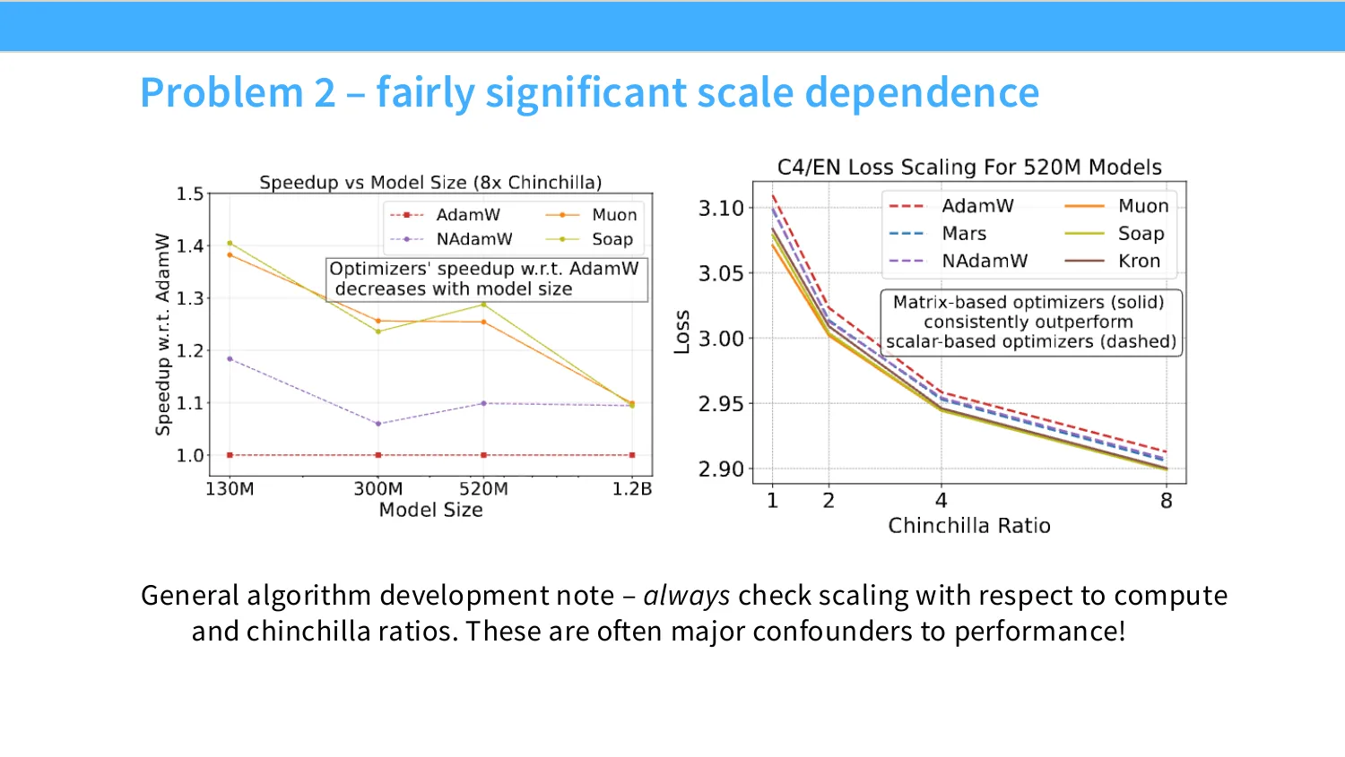
44:53 But maybe more relevant to the discussion in this class right now is the scale dependence of these things. And I think this is a good sort of case study and example. of how to really think about algorithm development as a function of scale. Because to me, you know, there are two variables that are always important when thinking about scale, and this paper exposes to some ex- to most extent like both of them. so one axis is compute, and you know if you're fixing the compute, oh sorry, if you're fixing the model size to data ratio, like the two are coupled together. Then this is essentially a compute axis on the x axis here, right? So you always want to, you know, whenever you're doing a study, you know, essentially scale up the compute and look at the trends as a function of of scale. And we see right here that if we look at the relative speed up between Adam, which is at 1.0 by definition, and all these other alternatives, we see that you know muon is really good at small scale. #

45:49 and that gain sort of diminishing down, diminishes down as we increase in scale. That's that's not really necessarilyum, the picture that you wanna see. There's another axis that you should always be vigilant of if you're doing algorithm development. And the other one that you should be vigilant of is the Chincilla ratio. So the Chincilla ratio can be thought ofuh, It is the ratio between, you know, how much data you have and the amount of model you have, right? And this is a really really really important parameter, because some algorithms work well in kind of the over parameterized case, where you have a way bigger model than you have lots of data, right? Maybe your your algorithmuh, Add some implicit regularization, right? Or maybe it, you know, is data inefficient, but it works well because of compute reasons, right? So, you know, some algorithms might work well at a small tilde ratio case. #

46:35 In contrast, you know, other algorithms might work well in the large chandler ratio case where you have lots of data per per unit parameter, right? Because you can pack knowledge more efficiently into the parameters, right? so this is a big big big confounder. even papers that i think have pretty good hygiene in doing scaling experiments on the model size axis, often neglect to or just don't have the compute to sort of study the chinchilla sort of token to to parameter ratio. and this turns out to be surprisingly important a lot of time. in this case, it's not. in this case, you know, you see that the optimizer sort of gains are Pretty consistent, the ratios between all the lines are the same at different chinchilla ratios. But this is not always the case. You always want to be vigilant about both of these scaling factors. #

47:20 That's quite important. #

47:23 And then I'm gonna you know also point out, you know, if you have a new algorithm or a new setting, right? Establishing scaling is quite non-negotiable, right? So, I've taken this from one ofuh, Will held who was working with Maren, which was you know, Percy's open source language model training project. And there, you know, they were basically trying to prove out a particular set of hyperparameters. This is even like a new algorithm. So this is cautious Adam C, which is like an Adam variant. Square root backside scaling, and a and a bunch of other sort of standard looking things. And you know they're doing essentially the same sort of chinchilla analysis that you've seen all the other papers do. But because this is not necessarily a paper, this is a bunch of you know people doing experiments. #

48:06 You don't just publish the the successful one, you know they have the niceness of publishing their failed runs. And the example here is that they're doing basically standard chinchilla stuff. And it's looking great. If you if you go up to this dashed vertical line at 10 to the 20 something, you know this is a this is a really beautiful looking scaling law to hear. And then you know as you scale up, it's like, well, it's a little bit worse, it's a lot worse, and then wow, now that run is not so good anymore, right? So it's just totally blown up on you. And the point here is that, you know, even good looking scaling trends for many orders of magnitude can suddenly kind of bite you, right? Like it can deviate from linear, and then it can then, you know, kind of blow up immediately. And in their case, you know, the the fix here Is just picking more careful mu p style prioritizations. #

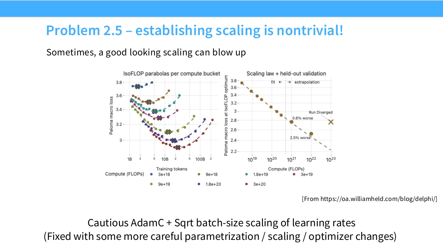
48:51 Optimizer changes, they switch to a pretty a different kind of optimizer, and you know they get nicer scaling across border orders in magnitude. But the point here Is to say, you know, when I go back here and I say okay, well, you should all do scaling experiments, you should scale all your learning rates and so on. That's not easy, right? You you end up fairly non trivial fraction of the time with pots that look like this. And it's all kind of horrible, and you're not quite sure what has gone wrong. #

07 Muon 优化器

49:19 OK. #

49:21 And then so the last thing, I wanna end with is just talking a little bit about Mewtwo, and sort of, you know, the closing up out the Mewtwo Mewtwo story. So, you know, I I feel like I have to talk about Mewtwo in a little bit more detail than I already have. Just because it's beginning to be integrated into a large scale model training runs. That's kind of the inclusion criteria for a lot of you know new research topics for the class, you know has it been in a big training run? And mu on now checks that mark, and it's also just kind of an interesting algorithm, so I'll mention it, and talk about it for a few minutes, and then move on. So, in gradient descent, we usually have a fairly simple. li-, you can ignore line four for the mo-, or sorry, line five for the moment. And then you're going to get roughly a standard, you know, momentum based optimizer, right? I take a gradient. #

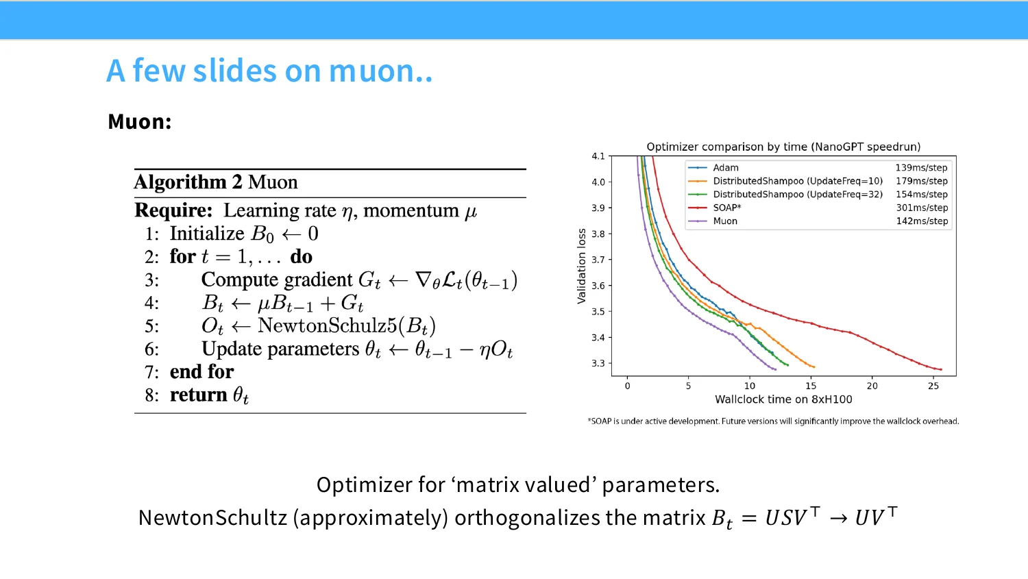
50:10 I added to BFT, this my momentum step, right? So I I in continue my momentum from before with parameter mu, and then I update my parameters based on this momentum gradient. Very standard, you know momentum gradient stuff. But then I think the really interesting, and to me at least a bit of an out of the box set of ideas is to say, well, you know gradients have this property that they treat all the parameters of the same. But we know that not all the parameters in language model or even the deep neural network are the same. Some parameters are like vector parameters, like they belong to the RMS norm. Some parameters are matrix parameters, like for the attention or for MLPs, right? And matrix parameters are probably different than vector parameters, and so that's kind of the starting point for this idea, and I think a really interesting one. And so the one thing that you could do about matrix parameters is you can start to look at their spectra, right? #

51:04 Like they are matrices. Matrices have eigenvalues and singular values. And so you can do things to the singular values, and so, what you do here in in nuon is this fairly simple idea. You compute a gradient, you take a momentum step, and now I take my update b of t. And instead of directly applying it to my parameters in line six, what I'm gonna do is I'm gonna do this Newton-Schultz thing, Newton-Schultz 5, to be specific. And what that is is it's gonna orthogonalize the B of T matrix. And so I've written the operation down there on the bottom. You know, let's say I take B of T, I write it as singular value decomposition, USV transpose, and then I make all of my singular values one, right? So, if my singular values are really big, I'll shrink them back to unit. #

51:48 If they're really small, expand them back up to being unit, and then I take UV transpose, and that's my new update that I'm going to apply, right? If you want intuition for this, and you already have intuition for something like Adam Grad, or these other, or Adam even. In Adam Grad or Adam, you're gonna divide by kind of the size of the gradient, right? So every coordinate is roughly gonna be the same size. in nuon, you were operating in the spectral norm instead, so every kind of direction is going to be unit size. And notice that this only makes sense for a matrix. I can only define this notion of a of a singular value decomposition for a matrix valued b of t, right? So, the interesting thing about mu on is it's a matrix optimizer. So you apply it to these matrix valued parameters, and for the vector valued ones, you know you might still use something like Adam W. #

52:36 Right, cause those don't really have any sort of interaction with the Newton-Schulz term. Oh, also, Newton-Schulz is a is a approximation to that operation that only uses matrix multiplications, right? So it's systems efficient. And not for exactly the the orthogonalization. But okay, like why have I spent you know all this time talking about Muon? Well, first of all, it's very you know powerful for things like the nano GPT speed run. It was discovered for this you know set of things. And so you might think that it works well. As I said in the previous slide, you know, there have been some scaling studies that have argued that the gain for muon sort of decreases. #

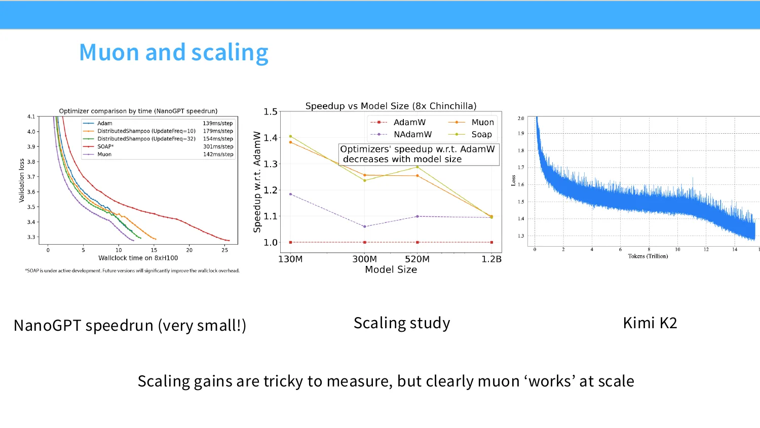
53:13 As scale goes up, but then you know I kind of wanna close off this story, which you know, I think initially this came out, and I was like, wow! Nuance kind of interesting, I wonder if anyone will scale it up. And then Kaya and other others scaled up Mew on, and they said, well, maybe it doesn't work super well. And I thought the story was kind of closed here. I was like, well, maybe this is done. No one will spend the big compute to to scale this guy up to the full pre training size. And then kimi k two comes out, and that whole model is trained with muon, like fully with muon, with a few bells and whistles to prevent muon from like blowing up on you. They found a whole bunch of instability issues. But Kimi K two is an outstandingly good model, right? It's a very good model. #

53:54 And the training curves look you know reasonable. And so really what this suggests is like, well, you know, mu on work that scale, like, is it better than Adam? Kimi K two certainly doesn't have any ablation, so we will don't know at that scale, but it is certainly a valid and workable solution. And so, what's the point of the story, it's to say it's really hard to know whether something works at scale. It's very very hard. But thus far, a lot of like small scale experiments and transferring them up to large scale has been the way by which we do science, right? And so, you know, you still want to respect things like the nano GPT speed run. We learn quite a bit from that and get good ideas. And then eventually they make their way to the big models. #

54:33 We'll see if you know people continue to do ablations at big scale and really nail down you know is muon better than Adam W at scale and so on. Those are interesting questions. to which we don't yet have the answers. #

54:44 OK, I'll pause here for a moment. This is the end of my optimizer section. I want to make sure everyone's good, also especially because I I was talking about muon, and that's a whole new can of worms. I haven't talked about much before. Yeah. OK. Great. Yeah, the question was, is a CD fast on GPUs? SVD is not fast on GPUs, but they're not doing SVD. #

55:09 What they're doing is Newton-Schulz. Newton-Schulz is a matrix multiply only finite iteration algorithm that approximates the process of orthogonalizing a matrix. So, there's like kind of several clever pieces here. One of them is kind of the idea of like treating it as a matrix on its own, and then there's this orthogonalization idea, and then there's the systems piece of doing it with Newton's method. So those are all like important interesting pieces. Yeah, back there. Are the hypervisors for the online share with some items for the different ones? Are the hypervisors shared? No, they're they're different, yeah. #

55:42 I think, you know, there are several people that have been working on this like nuance style line of work. And one of them, I think like Jeremy Bernstien, you know, I think he he's been saying like actually like every layer should have its own learning rate. You know, I think the the ultimate limit of this is like, you know, you go from, or even that's right, like every layer should have its own optimizer, right? The ultimate limit of this is to say every parameter in a transformer is different, why not have a different optimizer for each one of them, right? And so you would have Is you have a browser for each one of them as well? Which I do not want to do, but you know, that's maybe the feature of of optimization. Yes. Oh, the little bit of like, like for all the learning rate batch sizes, like they just consider like these two things, and then you pick Put that stuff of those, and then you kind of visit it to your other things. But do these things like Yeah, or or maybe the the version of the question that I interpreted was, you know, a lot of these people are just tuning learning rate and back flies and do the they use this on the grid. #

56:42 But presumably these things interact with a whole bunch of other hyperparameters. Aren't you worried about that? And I think in general, yes, you are worried about hyperparameter interactions. But realistically, they grow they grow exponentially, right? Like, this this is not a thing where you can grid out the whole space. And so, I think the the thing that people often do is they grade the stuff that's most concerning and most sensitive, and learning rates are very important. I think if you've you know ever tuned stuff, learning rates are the most important thing to tune. So they very aggressively go on that, and then stuff like weight decay, they might do a univariate sweep afterwards, right? #

08 muP：从推导到实践

57:14 To to be locally optimal with respect to those parameters. #

57:19 OK. #

57:22 All right, so the final part of this lecture is I want to talk about mu p. Mu p is a bit of a mysterious object, even with many papers written about it, and sort of in fact, even many implementations. I don't think all of them even agree on what the underlying math is, or what the underlying implementation should be. But there's a core set of ideas that are shared, and it does seem generally effective, and so I'll talk about Oh, my interpretation of the whole program, I love to call it. So, the goal hopefully is very clear, and I think this picture is the goal. The picture being well, if we increase the size of our model, in this case just with. Our optimal learning rate normally shifts, but ideally we want the optimal learning rate to be the same no matter what. I, that is the game that we would like to play, and the knobs that I'm willing to tune to do this is I'm willing to mess with the initializations at a per layer basis. I'm willing to mess with the learning rates on a per parameter basis as well. #

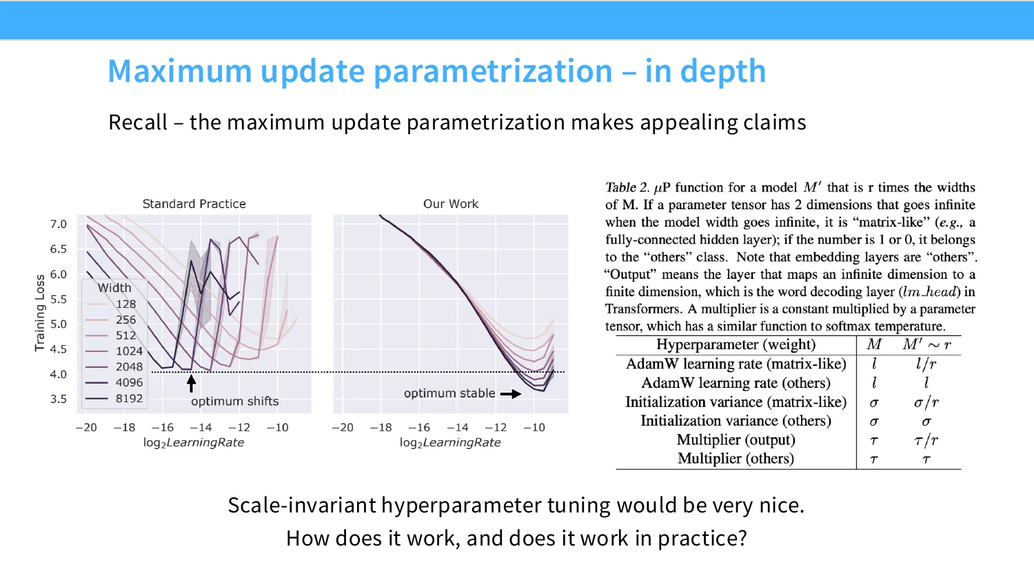
58:20 And then I'm sometimes willing to scale up or down things like residual connections, right, based on the size of my mom. OK, so that's the game that I'd like to play. And how well does it work in practice? There's been several papers that have studied these fairly extensively. Cerebras Cerebras, which is really a chip company. Also has a language model training arm, run by Hesse's of the Scaling Law, you know, paper fame. And they actually, I feel like they they do very interesting things, because they now are writing lots of papers about new p scaling of language models. And they have Cerebras GPT from a couple years ago, where they were training, you know, the 0.1 to 13B models using the usual Chinchilla recipe, but Also including a mu p variant, which they used to try to t- to tune the hyperparameters more effectively. #

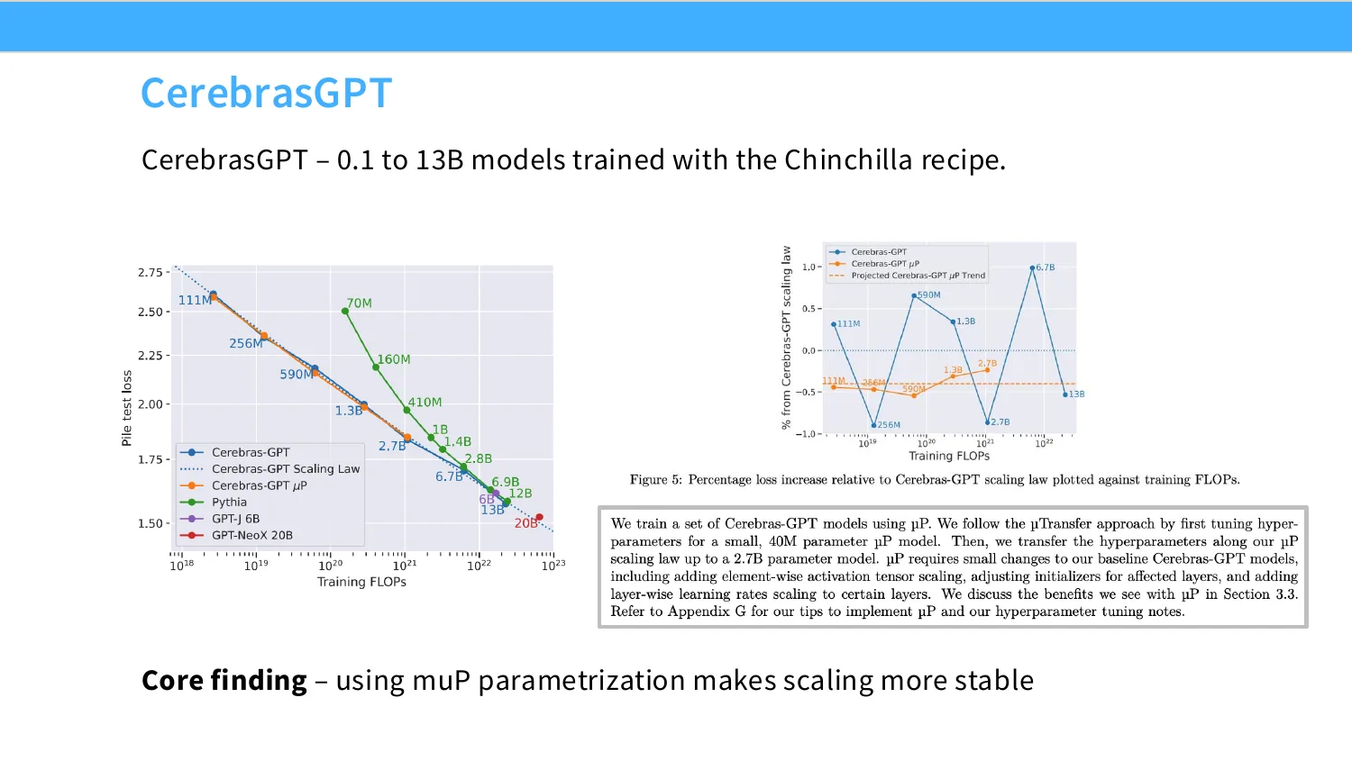
59:12 And I think one of the the nice things about this is they find that you know if they use the mu p primarization, then their scaling law fits are generally more stable. their their projected new p trends are you know almost right on the money for their actual models, whereas I think their their non new p models sort of fluctuated much more wildly in terms of the loss predictions. that they had, and so their claim was okay, new p is maybe a really good idea. so this is validated at scale, you saw many cpm and others, many people have trained models with new p variants. So, I could also talk a lot about, you know, training or examples of models trained with MuP. But I think maybe the more interesting thing for me to do right now is actually to talk about the conceptual foundations and the Math, sort of. #

1:00:02 And if you're interested in this, and you wanna read a somewhat accessible paper, I would recommend this one. This is the paper that I think For me was the clearest. There are several papers, Greg Yang who who kind of started this research program has a series of papers, I'll call tensor programs. I find them somewhat inscrutable. Jeremy Bernstein, you know, who was also working on the muon stuff, has written this nice sort of re-, not recap paper, like a like a review paper, sort of putting it into a different framework. which I think is very accessible. And there are several others by physicist that are also interesting in terms of explaining what mupe is. The the sergei's people actually do a bit of that as well. OK, but anyway, returning to this paper, the core idea of mupe is based off of two kind of assertions. #

1:00:46 Right, and this is a very physicist way of thinking about this. So, if I make my network big, let's say I'm only changing the width for now, right? I'm making the width of my network big. I'm gonna assert two invariants that should hold as I do the scaling limit. First of all, the activations at initialization, so if I initialize my model, and I put in some random data, the activations should remain the same size roughly as a function of the network, right? So if they blow up with the network size, or they shrink to zero with the network size, I've chosen a wrong prim trialization. That kind of makes sense, right? My activation should be roughly the same scale. regardless of the size of my network. #

1:01:24 Now, after one gradient step, the change in my activation should be O of one, right? So this is what people call feature learning. So feature learning means, if I take a gradient step, things in my network change a significant amount, and that this amount should be a fixed function of the width of the network. In case you know some of you are theorists right? You know you might be familiar with neural tangent kernels. Neural tangent kernels would have a very different behavior. Those would be the kinds of things where the changing activations actually vanish as a function of the of the network with, and you don't want that because you do want the network to change and learn features and do things even in the limit of your big sort of neural network. OK, so these two are the invariants. They. #

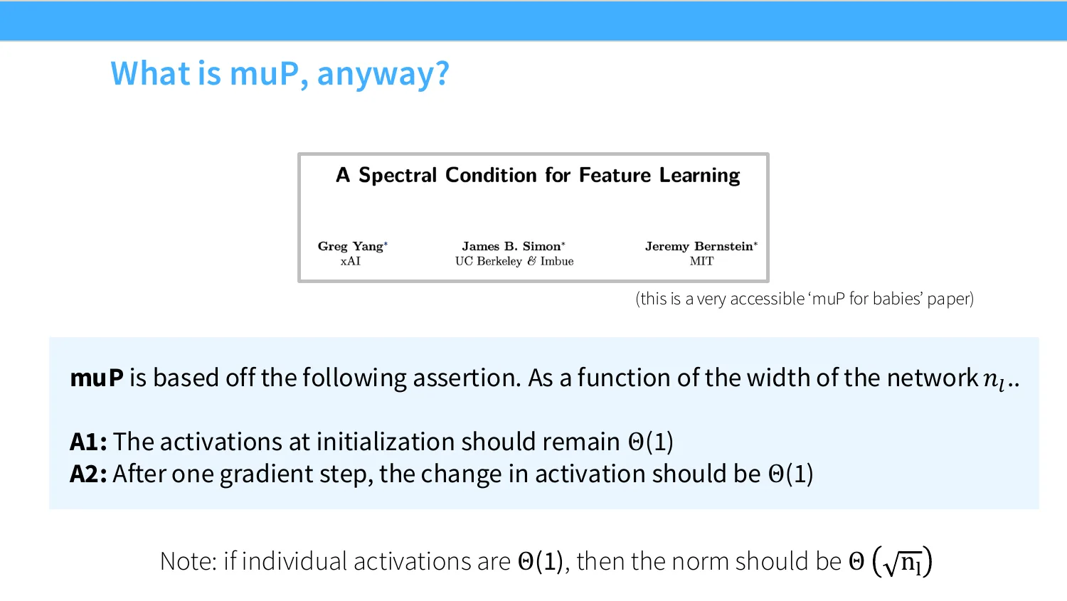
1:02:04 kind of make sense. They're basically saying activations and the change in the activations should remain roughly similar as a function of the width of the network. And then note that I'm gonna sometimes go back and forth the individual activations, which is this, and then the norm, which you know, if each activation is roughly O of one, the norm of the whole vector. or of activation should be square root of the Number of hidden units in that layer. #

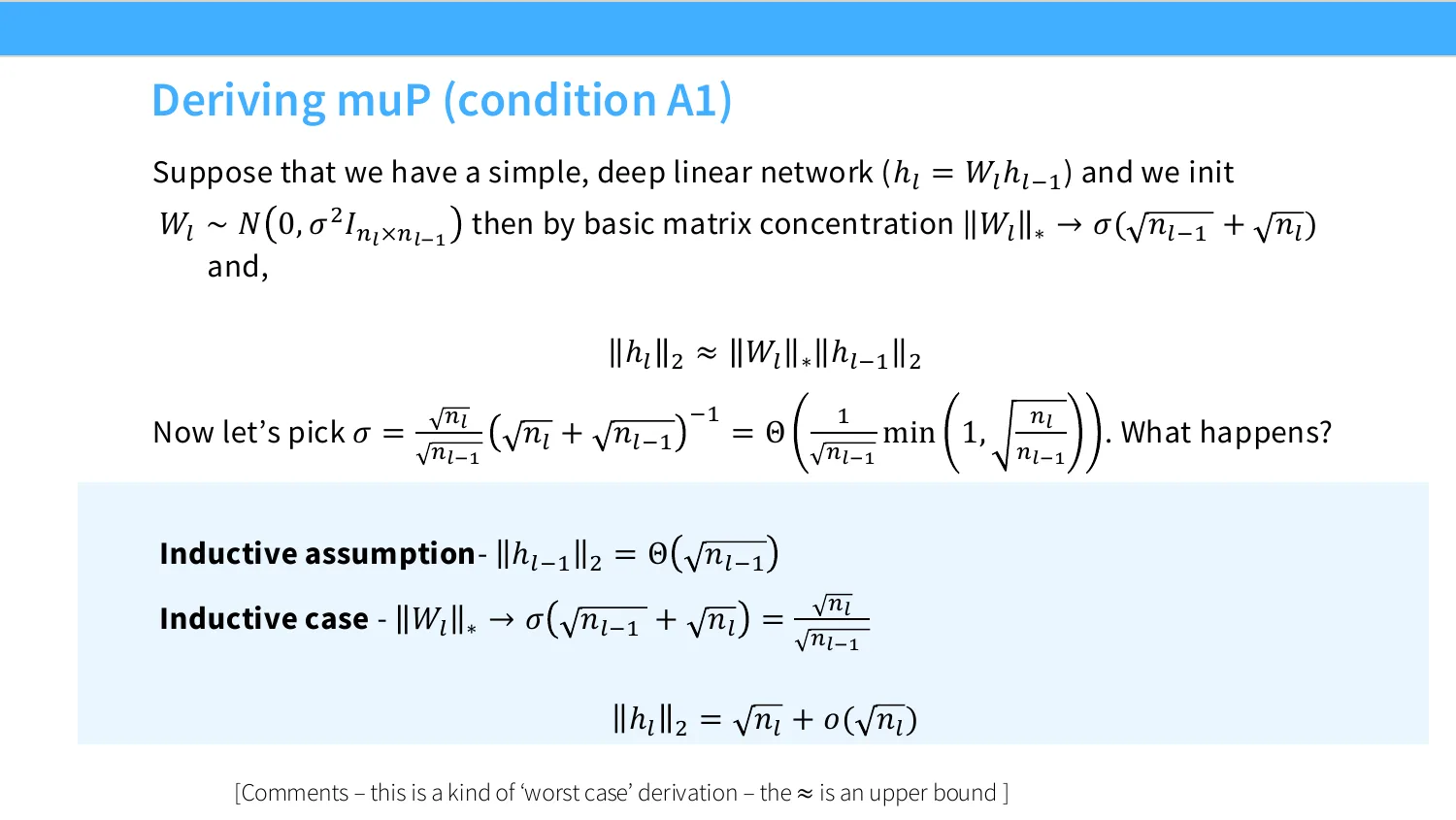
1:02:30 So, that's the main thing. Now, the thing about MUP is, it's kind of interesting, because it starts with, you know, this very simple and palatable set of assumptions. You might all agree that this is a reasonable thing to do. And then we're gonna make a a number of additional strong assumptions, but then in the end, we're gonna get a very simple set of scaling rules that drop out of this. So, remember what we wanna do is we wanna make sure that the activations that in it are roughly unit, so what do we do? Well, if we have a simple deep linear network, and we initialize all of our weights as a sigma squared, you know, scaled gaussian. Then what is gonna be kind of the spectral norm of this matrix? Well, you can write that down, right? I'm not gonna ask you to verify that, but that's you know Standard matrix concentration arguments for the operator norm of a random gaussian matrix. #

1:03:18 And then now note that in you know certain regimes where the fan out is, I think not much bigger than the fan in. You're gonna get that the output of the layer is kind of similar to the product of the input of the layer times the operator norm, right? This is always an upper bound, but this is you know approximate in certain high dimensional regions. now if this is true, now what can we do? well, we can solve for sigma to try to keep our activations the same across all of the layers and across all the width. So imagine that a layer at L minus one, I have sort of square root of L minus one activation, and this is remember, you know, consistent with this notation that you know, at least for this whole vector. I should have square root of n of l, right? So this is our our base case for induction. And then our inductive case says, well, you know, remember that I have this operator normal at layer L, which is this function of the fan in and the fan out. #

1:04:12 And so this is going to be equal to This, if I pick a particular sigma, so th- let's say this is the ansatz, I'm gonna assume that this is the answer, and then we'll see what happens to the induction. If I pick this as a hypothesis, and. I plug this into the sigma Notice that I get that the ratio of the operator norm is this, the ratio of the fan out over the sorry square root of the fan out over the square root of the fan in. and then I plug this back in here. And then I'm gonna get that the norm of the output is going to be equal to the square root of the number of units in my layer, plus some lower order terms that I not gonna bother to keep track of, right? So, you know, where the sigma came out of, I mean this is, you know, drawing it out of a hat, but we can kind of verify that if I, you know, plug this sort of noise initialization into my formula. Then essentially at every layer, the size of my activations is roughly equal to the square root of the number of hidden units at that layer, right? There are some assumptions made here, like this approximate equals, but this is like mostly a a legitimateuh, set of assumptions. So, condition A1 is pretty simple. #

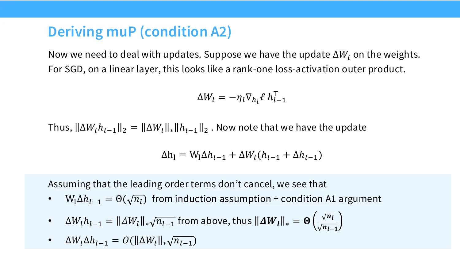
1:05:18 Condition A2 is a little bit hairier, to be honest. So, really, we need to deal with the updates now. And I'm only gonna consider the case of a single example in a batch for SGD for linear neural networks, so deep linear network. So what is this gonna look like? Well, the change In my weights for particular layer L, you know, if you think about how this is gonna behave, it's gonna be a rank one update between my gradient for the loss and sort of the activations. Right, this is true, you know, just because of the behavior of the backwards, right? The forwards is a rank one multiplication, the backwards is gonna be a rank one outer product. So now, you know this is the change in the weights, and now what is the change in the activations at that layer? Well, the change in the activations, you know I just take h equals w times hl minus one, and I expand this out, right? #

1:06:13 And expand this out into this formula, this is going to be exactly the change in the activation at layer l. And it's gonna have two terms, one that is sort of the direct term from changes in the activation at l minus one, and the cross term in some sense of what happens because my weights have changed. not just because the activations of the previous layer have changed, right? So there's two terms. to this to this update, and so this is kind of the change in the activation at layer l, and now what i'm going to do is i'm going to look through each of these three terms. I want each of these three terms to have the same order of magnitude. And I want that order of magnitude to be square root of n of l. Why is that? Remember that you know if I go back two slides, the condition that I want for a two is that after one gradient step, the change in activation should be o of one or omega of one. #

1:06:59 And so, if I want that to be true, then the norm of that layer should be square root of N L. And so, to do that, what I want is for each of these three terms to be to have that order of magnitude, and if that's true, and there's no cancellationsum, Then this, you know, is going to be the right order of magnitude. You can kind of see the sketchy pieces adding up, right? We're assuming things like no cancellations and so on. But this is giving us some interesting ways of thinking about the magnitude of each of these objects. So, you know, at this point, you know, the the right thing way to think about this is not like, okay, Tatsu is sitting here. Doing like rigorous mathematics, you know what I am doing here is I'm basically keeping track of all the orders of magnitude of all the terms, and I am saying that gi- given our assumptions, how big should these roughly be? It's like kind of physicist math, no offense to physicist. This was developed by physicist in this way, okay? #

1:07:48 okay, so now really, oh sorry, go go back one slide just to to make all this clear. So the first term, this comes by almost assumption, right? It's kind of the inductive assumption. We assume that delta h of l minus one has the right order of magnitude, right? So this comes for free. These other two terms, these are trickier. We have these terms that multiply the change in my weights in operator norm times square root of L minus one. And so, because these two are the sort of order of magnitude of both of these terms, We kind of know how big this delta l needs to be, right? We can solve for this because we know that this left hand side needs to be square root n l, and then we have this term, so we solve for this operator norm, and that's exactly this quantity, right? #

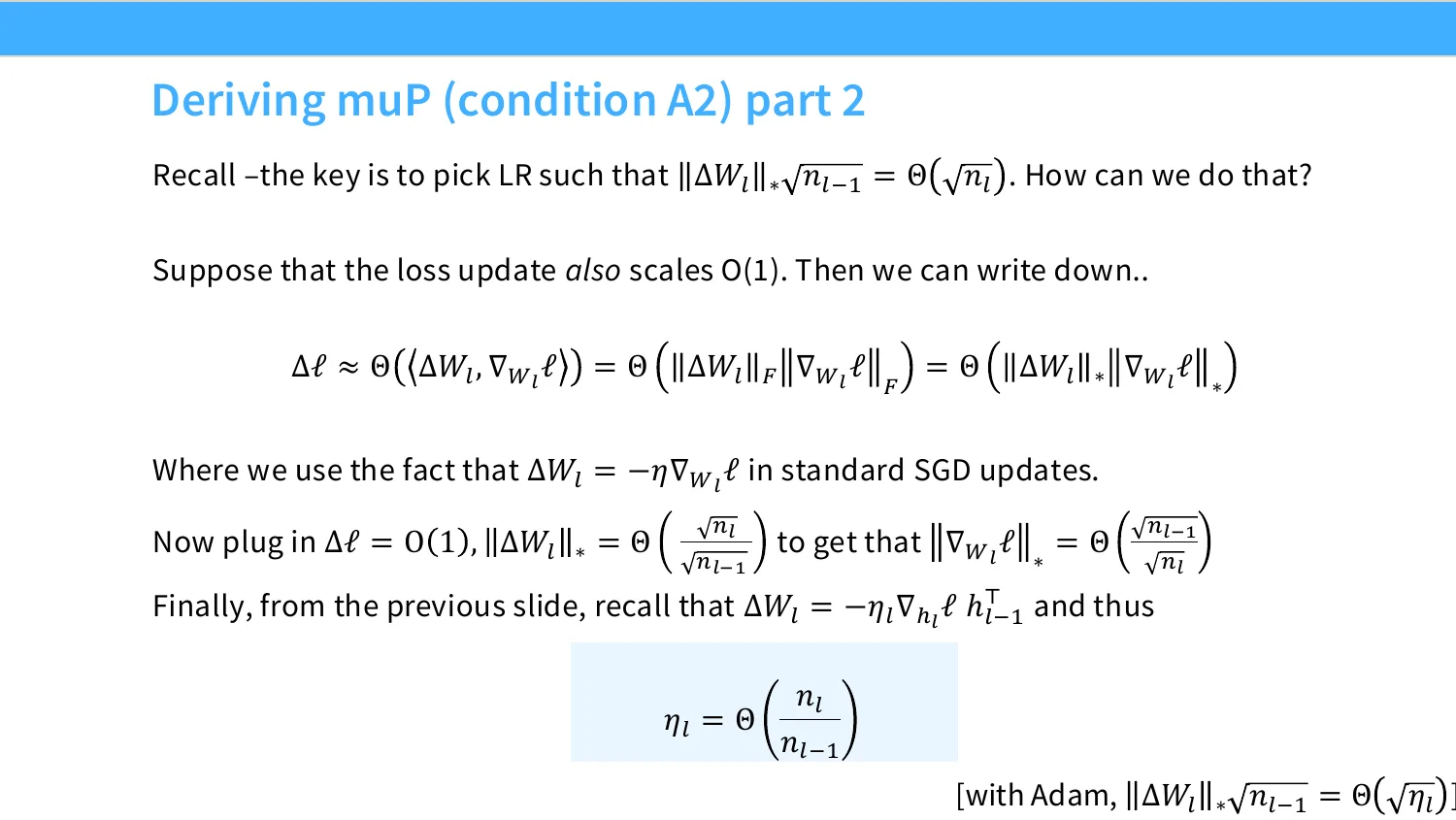
1:08:30 So, so this is gonna be the goal for the next slide. I wanna make, I wanna try to figure out what kinds of learning rates are going to give me an update that's roughly scaled as the square root of the fan out over the square root of the fan in. That's the goal, right? As I said, after I pick a learning rate, this should roughly be a true. So how can we do that? Well, we're gonna make yet another assumption, and this is probably the least palatable of the assumptions in my opinion. Which is that we're gonna assume that the you know the loss update is going to be scaled by unit. In other words, you know we're going to assume that you know our model is actually making some appreciable non trivial progress as a function of scale, and that that's roughly similar. Not quite sure that's palatable to me, but that is yet another assumption. #

1:09:14 So we throw that down, but now the the point of this assumption is that if this is true, the rest of the math works out quite cleanly. Because the change in the loss is you know the product of my gradient plus how much my weights change. This is Taylor approximation. And then because this is rank one, I can rewrite this thing as a Frobenius norm and as an operator norm. And so this right hand side now allows us to to get what we want. This is o of one, this term we want to be square root n l over square root l minus one, that's this term on the right here. And then finally, I have this gradient of l term. And this is gonna be square root of n l minus one over square root n l. And then so, now what a do I need? #

1:09:54 Well, the a that I need is going to be solving for this quantity, which is the ratio of these two guys. #

1:10:02 So, we made this one assumption that the left hand side of this is O of one, and then we've solved for all the quantities, and we've ended up with a fan out over fan in ratio for a learning rate for a layer. For one side note that I'll make is that for Adam, because of kind of the changes in in some of this, you're gonna get like a one over n l minus one scaling, which I'll all mention here. OK, so I've walked through a bunch of kind of hopefully intuitive looking scaling arguments for various components. But in the end, maybe you are interested in like what does this mean? What does this do for me? What this means is that we're gonna change how we set our initializations and learning rates a little bit. So, our initialization is going to look like, so for mu p, the blue box is kind of what we do. Our initialization is going to be one over square root n l minus one. Times a component that is one over the square root fan out over fan in. #

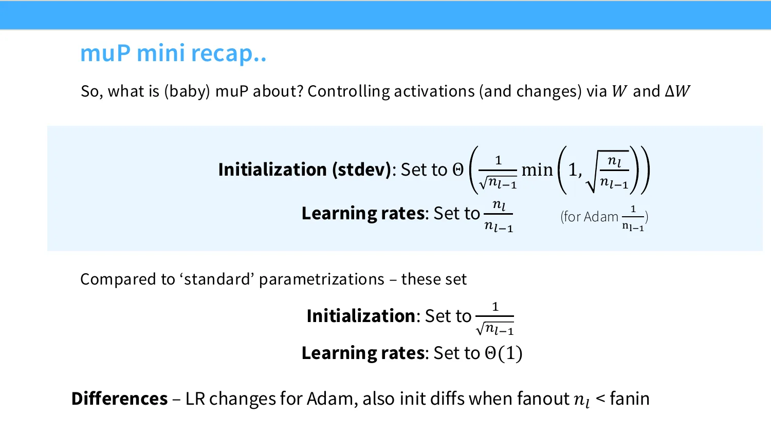
1:10:57 So if this is one, then this is equivalent to the usual initialization. This is the standard parameterization. But if this ratio is not smaller than one, then you get basically something different. You get something that's closer to the square root fan out over fan in. The learning rate normally you would set to be a constant as a function of your model size. But you would want to set this to the ratio of fan out and fan in. And maybe more interestingly for Adam, this whole thing is a little bit more different. I'm not gonna even touch the derivation for that, where you drop this one over an l term, and you get one over the fan in. As kind of the layer specific learning rate, and so basically layers that have big fanins for Adam get smaller learning rates. #

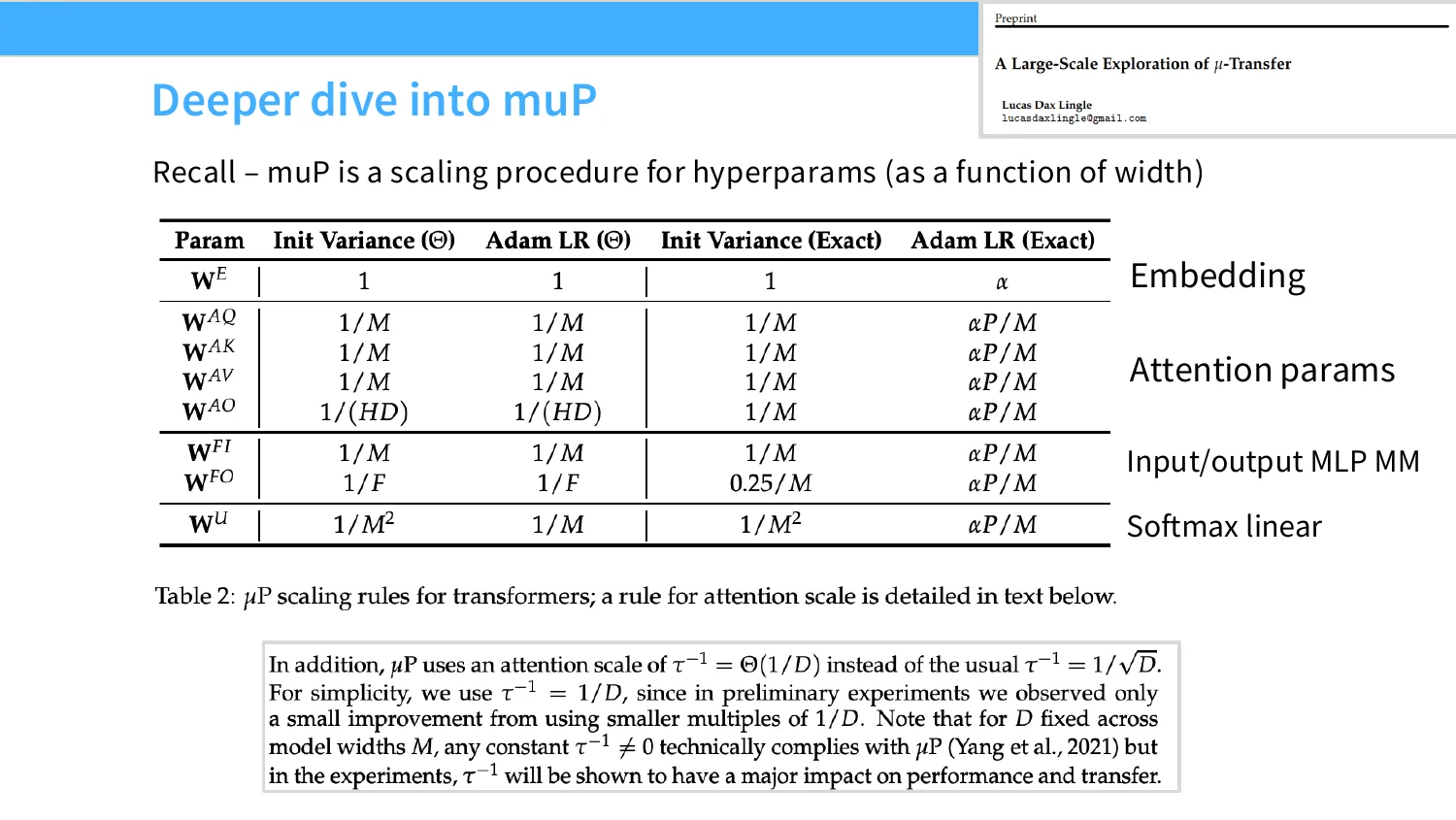
1:11:39 It allows you to have these layer adaptive learning rates that are quite interesting. OK, so that was kind of the derivation of mu p. Maybe you know, I I went through a lot of details, so I do wanna maybe talk about what the high level point of that was. And the high level point of that is, new PS sort of an argument is very interesting. Not only is there like actual useful stuff, the way in which you get to the algorithm is itself interesting, because it's this very different kind of math, in which you're saying okay. You know, I'm gonna take a scaling limit of my network, and then I assert some invariance about my network, and then I'm gonna make additional assumptions, and then I'm gonna try to figure out what the constraints on my sort of hyperparameters are. And the constraints essentially give you certain kinds of scaling limits on your hyperparameters as well. Right? So this is a general principle for coming up with different kinds of algorithms or hyperparameter scalings. #

1:12:30 I think which are probably very different than what you're used to, in CS or ML training. #

09 muP 的复现与鲁棒性边界

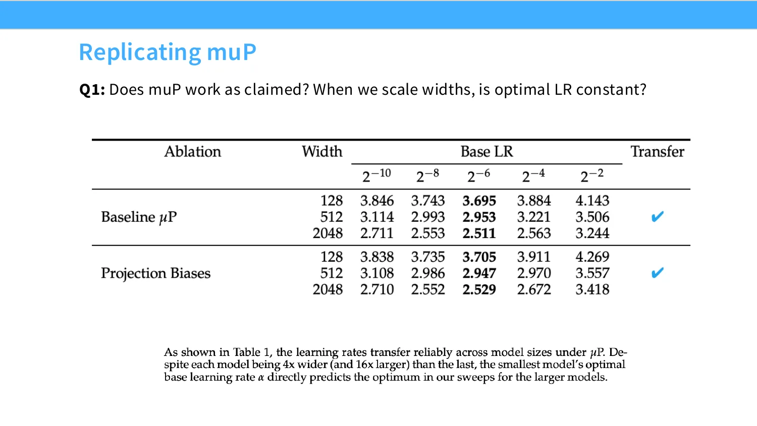
1:12:35 So, okay, that was the mu p derivation. I wanna close out on the mu p part with just a few like empirical things. There's a interesting paper by a a independent researcher, on basically stress testing MUP in lots of different ways. And MUP can be, you know, thought of as a as a proce- procedure for tuning hyperparameters. And so, you know, depending on how you do things like, you know, Adam is gonna have a certain learning rate as a function of different components of the network. So you have an embedding parameter. Attention parameters, input, output, MLPs, or softmax linears, all of those are gonna have different kinds of scalings, under mu p, as well as not mu p scaling rules. And the interesting thing here is that particular paper, you know, replicated a bunch of the MuP results for language models trained at different scales. And maybe unsurprisingly, he found, you know, almost the headline result from MiniCPM and others. #

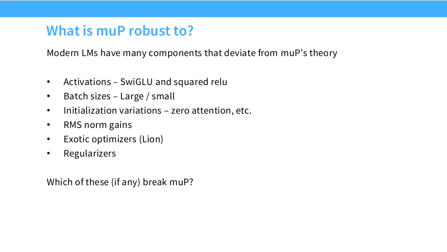
1:13:35 Which is that if you get the mu p right, and you're only scaling with, in this case, in a very controlled way, you get exactly the learning rate optimality and variance that you know. baseline mu p, or just looking at kind of a variant of mu p that sort of tracks projection biases for attention. both of those transfer very nicely. but then you might ask you know, basically, there's a lot of things in the real world that mupe does not handle, right? Like technically, SqueezeLube does not fit into mu p. Neither does, you know, initial variations initialization or RMS norm, or if you really mess with your optimizer, that'll mess that up too. And so you might ask like which of these like, you know, things that are not allowed by the theory really break New P? And actually, for the most part, these mostly work with New P, but some of the things that don't work Is if you you know learn the gain term in RMS norm. This turns out to break newbie. #

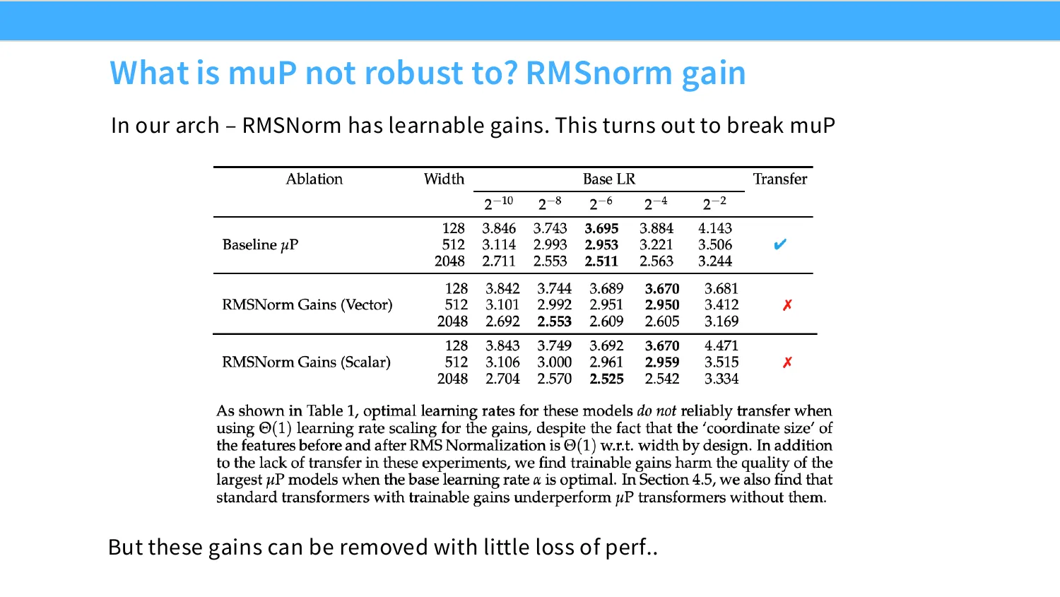
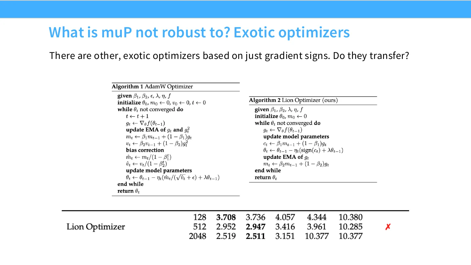
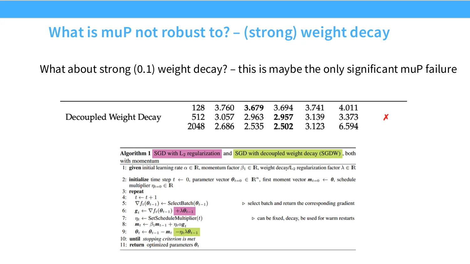
1:14:32 Although these can be removed in many cases without necessarily hurting you, and so maybe it's not such a bad idea. but this does seem to break mu p. it also seems to break if you use more exotic optimizers like lion, which basically rely on the sign of the gradient. and this is sign gradient is kind of like a c- a spiritually similar to mu on and other ideas, and so There might be other interesting things that break with mu p as well. Finally, the thing that seems most concerning is that if you do large decoupled weight decay, you end up with a significant mu p failure. So this is maybe the one stress test that it does fail. #

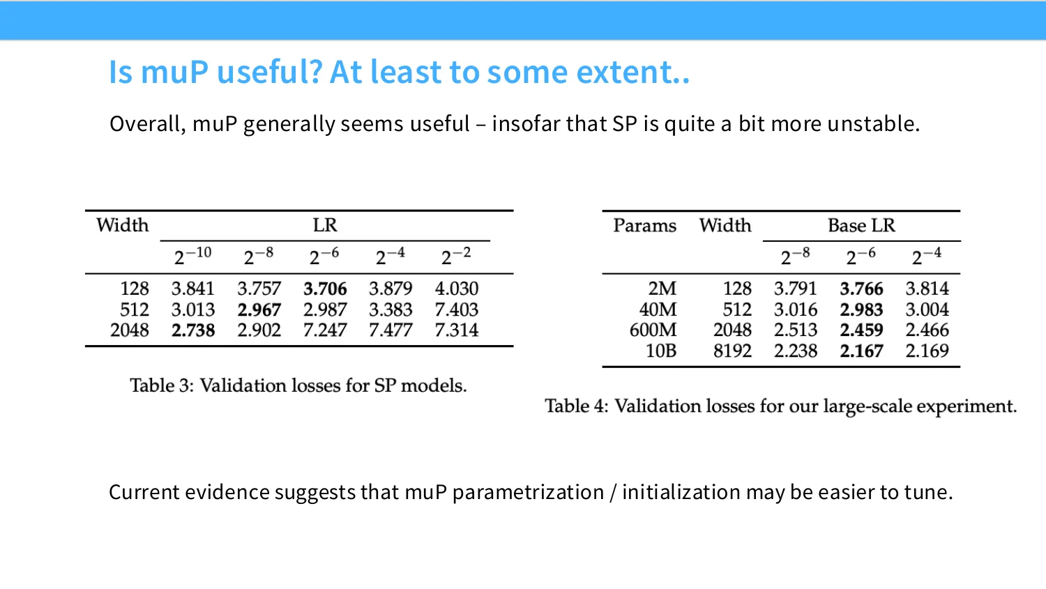
1:15:11 But to close out this final section, you know, you might in the end ask like, is new p useful? And if you really want to stabilize your learning rates, it is actually pretty useful. There's a lot of experiments of this form where, you know, if you increase the width Your optimal learning rate shifts very predictably, but you know very greatly as a function of scale, whereas in mu p it doesn't. And so it's one of the many tools in the toolkit to try to control hyperparameter drift as a function of scale. I think it's an interesting open area of research. It's not really sort of you know done and dusted, and like this is the one right thing to do. #

10 小结：scaling in the wild

1:15:44 But there's a lot of promise in sort of the MuPied initialization program. There's also a lot of promise in just fitting scaling laws as well. #

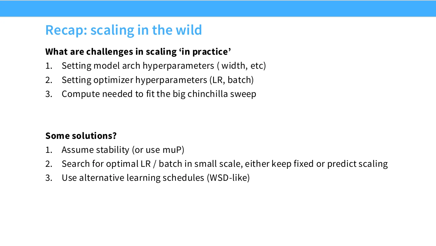
1:15:52 OK, so final thing I wanna close with, you know, scaling in the wild is very tricky. As I sort of mentioned in one of my replies, you know, I think the initial presentation of scaling laws makes it sound like a science, right? Like It's like, yes, draw this line, do these procedures, and you will know for sure what will happen at scale. But I think in reality, it's a lot more messy and a lot more unknown than that. You know, there are lots of things that people do use and practice scaling loss for, like picking architectures, picking optimizers, picking hyperparameters, right? All these things are things that people do with scaling loss. But there is really an art to it, in the sense of, you don't really know if it's truly gonna extrapolate forever. You want to do sort of reasonable things to maximize the chances of success, right? And so there's lots of solutions that people have. #

1:16:38 You can use mu p, you can search for the optimal learning rate, and all these other kinds of things. And these are ways of controlling hyperparameter drift, but there's no silver bullet yet. Maybe next year, there will be module that's like we solved it, but not quite yet. #

1:16:53 Great, thanks a lot. I can take questions afterwards. #